Aerospace Sensors Testing: How Solar Simulators Enhance Aerospace Sensor Testing

Flight is a wondrous miracle, one we all benefit from, whether it’s through air travel, GPS systems, weather monitoring, or indirectly through the gleaned knowledge from space exploration.

Regardless of the application, aerospace systems have to execute their jobs reliably, because the consequences of getting it wrong at 10,000 feet, in zero gravity or in a cold vacuum can be dire.

As a result, the aerospace industry relies heavily on a large number of sensors to continually monitor flight status and the surrounding environment.

These sensors must be reliable, and thoroughly tested on the ground prior to flight.

Sensors have to be robust enough so the failure of an individual component won’t jeopardize an entire flight or mission.

To reduce dependency on individual component failure, components are often incorporated several times redundantly into a design (and some design standards require this).  That means that any component’s weight may be multiplied several times when it’s finally implemented into a design.

Since a large amount of energy is required to bring something from ground level to high altitudes (or beyond), every gram of mass matters. Therefore there is ongoing pressure to have low-weight sensors, as well as to reduce the number of sensors required for measurements. Designers would like to have fewer sensors that can execute a variety of tasks with exceptional robustness.

A general trend in any aerospace application is to reduce sensor size and weight, and increase their efficiency.

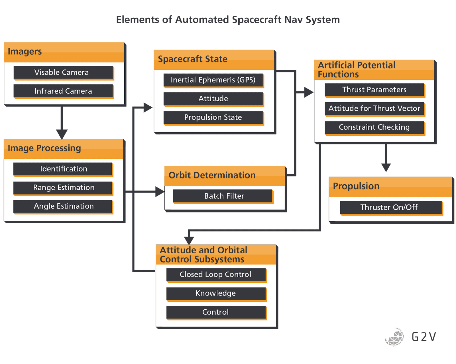
Even as the industry pushes toward having fewer sensors, however, there are still a wide range of tasks and functions that need to be carried out. For example, below is a proposed tree of functions, algorithms and instruments that would form part of an automated navigation system in a spacecraft:

In the field of remote sensing, a variety of sensor requirements and desired features exist simply because of the multi-faceted, cross-disciplinary nature encompassed by any work in mapping or remote detection.

Some of these remote sensor requirements and desires are captured in the table below, to give just a small sense of the industry requirements.

Sensors	Attributes
Ground Sensing and Navigation
Camera	Can image downward, forward, and off axis Can zoom Can automatically track specified item of interest Can autonomously create and return a mosaic of a given area
Spectrometer	Can image downard, forward, and off axis Can successfully image at wide field (to show general existence) and narrow field (to recognize location) Can automatically track specified item of interest Can autonomously create and return a 2D mosaic of a given area Can create overlay maps of different spectral images in parallel
Laser and/or Radar altimeter	Can image downward, forward, and off axis Could be used to image hydrothermal vents Could be used to image glacier areas covered by dust and dirt
Ground Penetrating Radar	Can image downard, forward and off axis Can autonomously create and return a 3D map of area Can return surface information up to 5 meters below the ground
Magnetometer	Could provide 2D and 3D models of magnetic variance Could be used to direct aircraft toward the existence of mineral deposits
Drop Probe	Ability to perform close up and micro imaging of material on ground Contact sensors capable of recognizing different chemical compounds Ability to provide data back to aerial vehicle Persistent beyond vehicle flight
Tetherbot Probe	Probe deployable on hillside allowing movement of sensors up and down the hill Includes cameras that can recognize rock types and micro image rocks Ability to provide data back to the vehicle Persistent beyond vehicle flight
Ground Penetrator Probe	Can penetrate 1-5 meters below surface when dropped from 100 meters Contains visual sensors Contains contact sensors to perform chemical processes
Atmospheric Environment Sensing
LIDAR	Can image downward, forward, and off axis Provides ranging from reflective surfaces Could provide backscatter data, allowing 2D and 3D models of terrain
Doppler Radar	Can provide advanced warning of turbulence, and high winds to allow advanced flight planning and maneuvering Can provide 3D maps of weather and atmospheric phenomena
Chemical Spectroscopy (methane, other chemicals)	Would provide information to control the aircraft toward altitudes or locations where specific chemicals exist Would provide 2D and 3D models of atmospheric chemicals Could provide 2D and 3D models that could be used to predict emissions emanating from ground sources

A wish list of features for different remote sensing applications, reproduced from https://doi.org/10.1117/12.595353

Any of these sensors used within the aerospace industry must perform to a high standard, which implies testing to minimize risk and ultimately achieve exceptional reliability and performance confidence.

Ground testing is a necessity for new aerospace designs, and accurate ground testing relies on ground tools and instrumentation that adequately reproduce expected in-flight conditions. Some reproduction of in-flight conditions involves flight load simulation, material static and fatigue, structural dynamics, acoustics.

Reliability and functional testing under the expected temperature, pressure, vibrational and illumination conditions is key.

Because so many aerospace sensors rely on visual, infrared or other spectral data, being able to account for a sensor’s interactions with the sun is paramount. 

In this article, we discuss how solar simulators can assist in the testing of a wide variety of aerospace sensors, and what features to look for in this industry application.

Validating Sensors for Attitude and Orbit Control  Systems

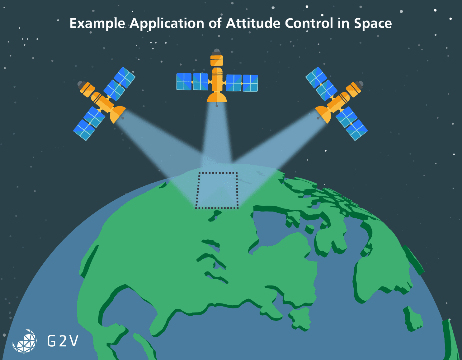
One key subsystem for almost any spacecraft is one that stabilizes and controls orientation and orbit. Known as the Attitude and Orbital Control Subsystem (AOCS), this system’s function is to maintain a spacecraft’s orientation, properly direct communication antennas, properly orientate solar arrays, and properly point cameras and instruments at their targets of interest.

One example of a key sensor in an AOCS system is a sun sensor or star tracker, which tracks the positions of nearby celestial objects in order to determine a spacecraft’s relative position and orientation. Other technologies commonly used for AOCS include gyros, magnetometers, gravity sensors, and IR detectors.

The overall determination of a spacecraft’s rotational attitude is achieved using banks of sensors.

Combining more sensor measurements in the AOCS generally improves accuracy.

However, it’s not enough to carry out these measurements occasionally – they must be executed more or less continuously throughout a mission so there is accurate data to inform the spacecraft’s next operation or task.  

The typical flow for AOCS system operation involves the following phases:

1. Acquisition: Getting a first estimate of orientation and movement
2. Coarse control: Starting to maintain a desired orientation
3. Fine control: Achieving full stabilization to permit higher-precision sensor pointing
4. Slew control: Intentionally changing orientation onto another target

As we execute more complex operations in space, the required accuracy increases, and so the performance requirements of AOCS sensors have been steadily increasing with time.

The precise details depend on the particular sensor in question. Generally, AOCS sensors are broken down into three sub-categories: rate sensors, coarse pointing sensors and fine pointing sensors.  

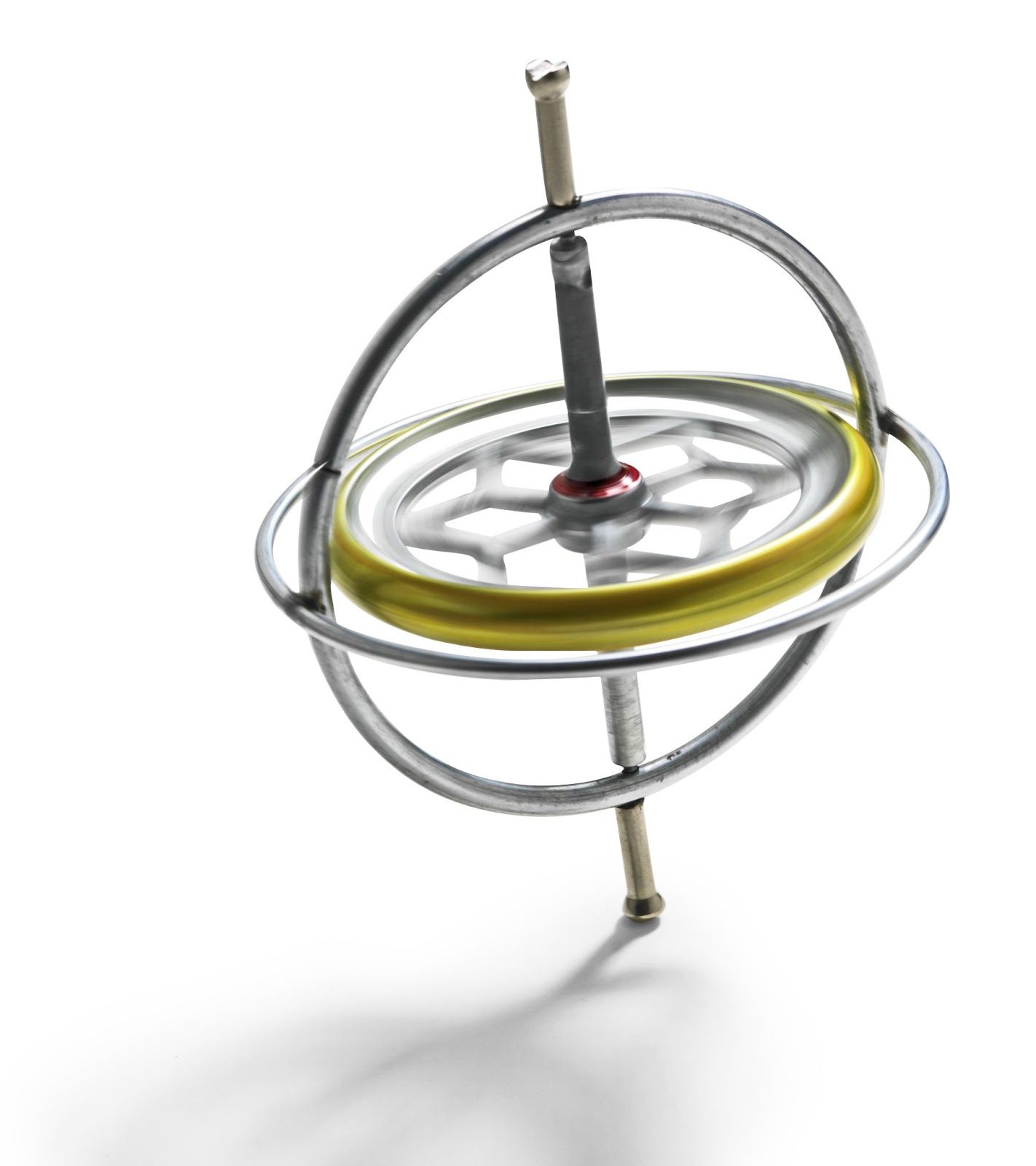
Rate sensors generally measure the spin rate of a spacecraft, and this task is typically achieved using gyroscopes.

Coarse control of pointing is usually done via sun sensors. These consist of solar cells and baffles, where differential signal levels on opposing solar cells will indicate relative alignment with the peak brightness from a desired celestial light source. Position-sensitive detectors (PSDs) of many kinds could be useful for this application, provided they can survive the harsh space environment.

Sun sensors are often hardwired into the emergency sun re-acquisition system, which serves to reorient a spacecraft to the sun when primary controls fail. This important role can’t be overstated. 

An unreliable sun sensor can lead to disruption of ongoing measurements, loss of communication, and/or loss of power by not accurately aligning to the sun for photoelectric energy capture. These impacts can, in the worst case, result in complete mission failure.

Sun sensors must therefore be designed and tested with the utmost rigour. 

Sometimes other bright objects such as the Earth are used to determine orientation. In this case, the planet’s edges are determined by signatures of thermal emission.

Sometimes GPS satellites are also used to determine attitude and orientation, because their multiple antennas can be used for triangulation. This strategy is limited to systems that only need a coarse attitude lock within 0.5 degrees, but it is low-cost and uses proven technology that’s likely already part of a craft’s design.

The general approach of GPS triangulation for attitude determination is to first obtain, through GPS measurements, the craft’s antenna locations in two coordinate systems. Once that information is known then the rotational orientation between the antennas can be determined via a series of mathematical coordinate transformations.

Fine pointing control in a spacecraft’s AOCS is usually achieved using a star camera. There are many designs of such sensors, but they basically consist of a series of lenses and a charge-coupled device (CCD) chip. The lenses form an image of the star field on the CCD chip, and from the locations of the stars the spacecraft’s orientation can be determined.

Typical star-camera sensors have accuracies of roughly 1 arcsecond, depending on the number of CCD pixels.

A summary of various sensor technologies for attitude determination is provided in the table below.

Various Sensor Technologies For Attitude Determination

Sensor Technology	Measurement Type	Limitations	Accuracy
Star Tracker	Three-axis attitude based on multiple vector measurements to different stars	Star needs to be visible	~1 arcsecond
Conventional sun sensor	Vector toward Sun	Sun needs to be visible	~1 arcminute
Magnetometer	Vector along magnetic field lines	Magnetic field needs to be present	~0.5 degrees
Gyroscope	Inertial change in three-axis attitude	Only relative angular measurements
Horizon sensor	Vector toward centre of Earth	Horizon needs to be visible	~0.1 degrees
Accelerometer	Vector toward centre of Earth	Needs to be in gravity field on ground or aircraft; onboard spacecraft will not work	~0.1 degrees
Multi-axes sun sensors	Multi-axes attitude based on vector toward Sun and rotational axis	Sun needs to be visible	~0.1 degrees

A summary of sensor technologies for attitude determination, reproduced from https://doi.org/10.1109/MAES.2016.150024

There are a variety of techniques to improve the accuracy of star cameras, such as deliberately defocusing to blur the stars and more accurately determine their centroids. Cooling also minimizes thermal background noise. On-board algorithms for processing the data are usually straightforward, with the majority of detailed and algorithmic processing carried out on the connected ground station.

One of the ways the pointing accuracy might be improved while minimizing the number and footprint of sensors is by relaxing some of the stringent model requirements for analysis combined with implementation of more elegant, flexible algorithms.

Elegant, accurate solutions are increasingly necessary as we venture farther into space. Even in typical space applications, for example, communication transmitters and receivers must have exceptional pointing accuracy of 0.03 arcseconds. 

These requirements are even more stringent and integral for deep space missions, which demand pointing accuracy on the order of a few microradians. The pointing of all communications equipment in turn depends on accurately knowing the orientation of the spacecraft, which is the entire function of the AOCS subsystem.

Any new techniques or AOCS sensors will therefore require increasingly rigorous testing. Next, we’ll discuss some of these typical test procedures for AOCS sensors.

Testing AOCS Sun Sensors

One important concern for any position-sensitive detector system is that their performance depends on the incident light’s spectrum.

Therefore, for spacecraft AOCS systems, it is usually best to try and test their response to the solar spectrum in space, AM0.

AOCS sun sensors are ultimately most dependent upon angle, however, since orientation is one of the primary outputs of the measurement system. Therefore an AOCS sensor test should focus primarily on establishing the angular resolution and angular uncertainties.

Doing the testing under the correct spectrum is more of a secondary concern, although a more accurate spectrum can play a role in reducing uncertainty in the sensor’s measured performance.

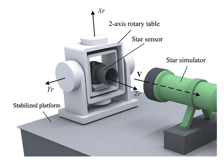
A typical AOCS sun sensor test would consist of placing the sensor beneath the irradiance of a solar simulator (Ortega et al., 2010).

After calibrating the solar simulator’s output to AM0, the position-sensitive detector (PSD) would then be tilted in both planes to generate a 2D contour of PSD as a function of tilt angle. From there, relative differential functions in both axes can be derived.

These functions then allow a user to determine tilt angle based on the measured outputs from the PSD.

For a more concrete example, let’s take the case of two photodiodes (equations and arguments pulled from (Ortega et al., 2010)).

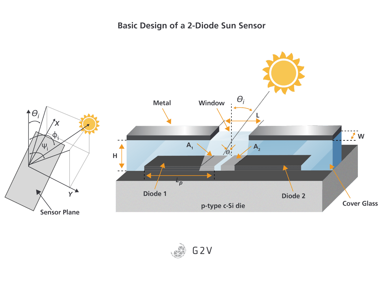
The photocurrents in the pair of photodiodes can be written as

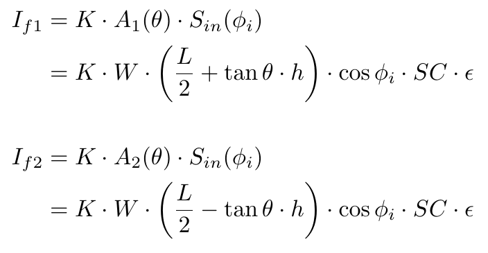
A relative differential function can then be defined as

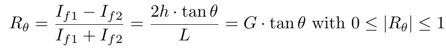
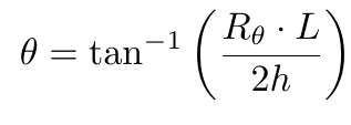
You can therefore determine the sun’s angle by measuring the amplitude of the two different signals, and using the following equation:

The same thing can be done in the other plane, where we have two additional sensors 3 and 4 (Note that you’ll have to use the appropriate L and h for those sensors, if they’re different).

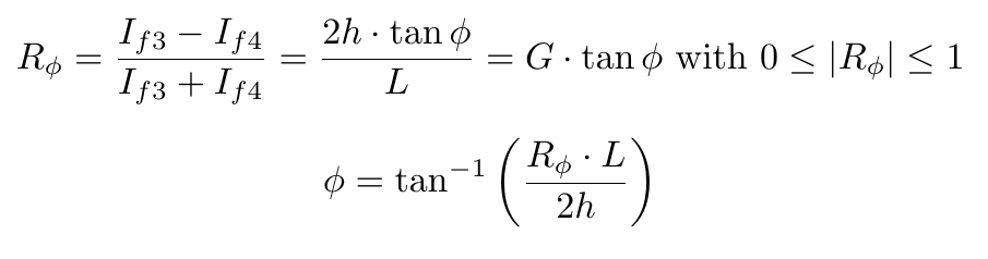
From this so-called relative differential equation (Ortega et al., 2010) we can see that the individual sensor noise limitations, as well as the physical dimensions of the setup, will determine the angular sensitivity of such a pointing sensor.

Generally one can map the response of all relevant photodiodes as a function of tilt angle, and this can be used to produce a calibration curve. Once that is done, a verification test is usually needed to check accuracy.

Random angles are set, and the predicted angles from the calibration curve are compared against the known angle settings for the stepper motors controlling the motion. This comparison yields an estimation of the accuracy of the angular measurement system.

While this example was relatively simple involving a small number of detectors, similar principles can be applied to test any sun sensor or star tracker.

Testing Visible Cameras For Orbital Manoeuvres

Imaging cameras play many roles in aerospace applications, and one important such role is for navigation and orbital manoeuvring. This role often falls under the purview of the AOCS subsystems, especially when, for example, they’re used in conjunction with active range finders such as LIDAR for range and angle estimates of relative positions.

However, the overall versatility of visible cameras mean they can also be used for a variety of mission-specific applications beyond spacecraft control. The umbrella for this wide array of applications is best encompassed by the term Space Situational Awareness (SSA) — knowing the location of objects within and beyond Earth orbit to a desired accuracy.

The three subcategories of SSA are

• Space Surveillance and Tracking (SST) of human-created objects (for a specific application of this, see our case study with the French space agency CNES)
• Space Weathering monitoring
• Near-Earth Object (NEO) monitoring

Visible imaging can be useful for all these areas of SSA. For example, the optical navigation camera telescope (ONC-T) onboard the Hayabusa2 spacecraft was designed to optically navigate, as well as to map the mineralogical and physical properties of its intended target, the asteroid Ryugu. The imaging data it received was used to determine the ideal landing location.

Traditionally, SSA was achieved via measurements from ground-based instruments (such as radar).

However, more and more spacecraft use in-orbit sensing and inspection tools which require a higher level of automation and detection. Researchers would really like to autonomously manoeuvre and inspect in-orbit objects to help reduce the chance of accidental collisions resulting in Kessler syndrome. With orbital crowding and a push toward spacecraft maintenance comes an increasing need for proximity operations.  

Two examples of autonomously operating spacecraft are from the Air Force Research Laboratory (AFRL): the XSS-10 microsat, and the DARPA Orbital Express mission.

The XSS-10 used a visible camera system (VCS) along with rate gyros and accelerometers to estimate its relative position to another spacecraft. The DARPA Orbital Express mission involved a spacecraft servicing demonstrator called ASTRO, and its Autonomous Rendezvous and Capture Sensor System (ARCSS) which was the main technology for navigation and rendezvous. The ARCSS instrument suite incorporated a visible camera, infrared camera, and laser rangefinder.

Visible cameras are crucial for the future of space operations, and they’re going to be increasingly relied upon to provide accurate information. Testing them, as before with the AOCS sun sensors, is vital.

Error Sources and Tests for Navigation-Focused Visible Cameras

Visible cameras that use image processing algorithms to yield positional information generally go through three main phases:

1. Target identification
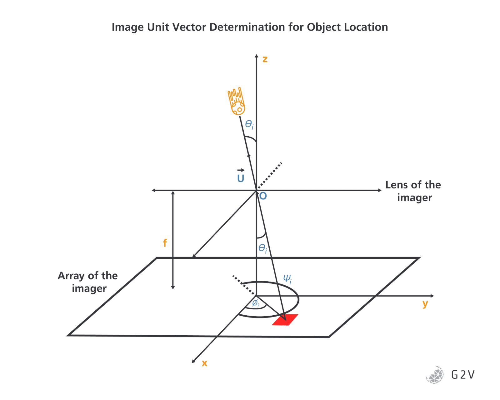
2. Vector determination
3. Range estimation

The identification stage relies on finding groups of pixels of a certain intensity. This is roughly analogous to a measure of visible radiance (for visible cameras) and/or temperature (for thermal cameras). The intensity profile is used to identify what kind of object a target might be, while its center of brightness can be used to begin determining the vector.

Stray light sources contribute to noise, and the Sun’s position relative to the illuminated object can impact the amplitude as well as the distribution of reflected light from an object. 

A solar simulator can be useful for testing a variety of Sun-object configurations, and assessing how much stray light ultimately interferes with the desired signal. Knowing the Sun’s impact on the error in the center of brightness estimate, for example, can ultimately provide a confidence level for the object vector determination shown below.

Range is usually estimated from the ratio of the imaged object area compared to its expected area. Obviously for this to work, you have to have pre-knowledge of the object you’re looking at.

A key improvement in the future will be to be able to do this estimation without object pre-knowledge.

Range estimation consists of four phases:

1. Major and minor axes determination: figuring out the long and short dimensions of an image.
2. Calculating the ratio between major and minor axes
3. Estimating the area of the object, and its uncertainty
4. Estimating the range, and its uncertainty

Testing each of these phases, for the sizes and shapes of anticipated objects, is highly beneficial for mitigating mission risk.

Researchers want to assess how well their camera can image a uniform light source (such as that from a solar simulator or an integrating sphere) , in order to remove the camera’s response function from data analysis and ensure that any shape features are related to the object being imaged and not the optics. This is often referred to as flat-field correction.

An example of the normalized profile (i.e. flat-field response) for a specific wavelength band is shown below.

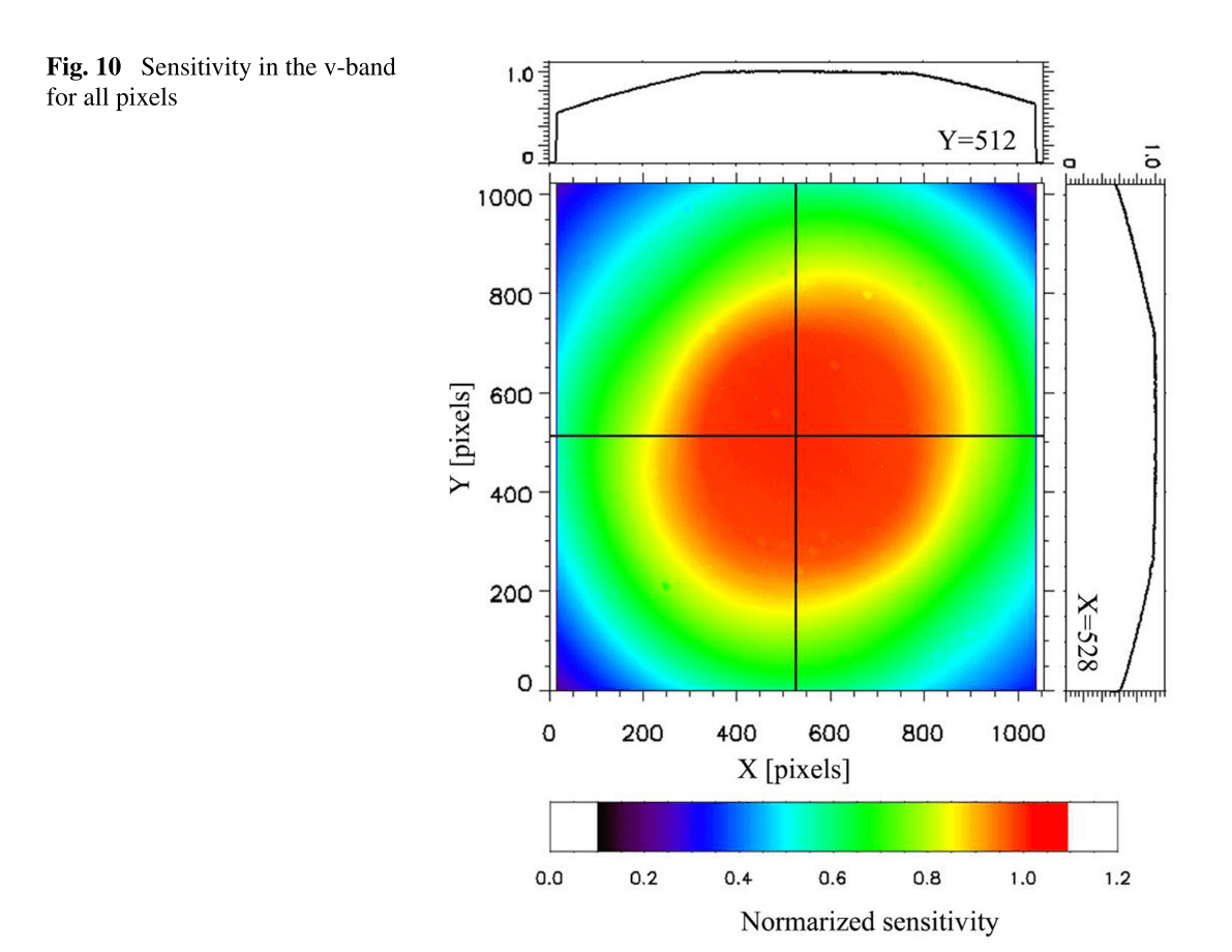
It’s not sufficient to know this for a single wavelength band, however. Since a visible camera’s response to light will be wavelength-dependent, some of the errors and flat-field response described above will also be wavelength-dependent. Having a light source that allows you to fully assess this wavelength sensitivity can provide early indications for whether or not a camera meets specifications.

Generating the same dataset above for all a camera’s spectral bins can yield, for example, a plot of the average spectral sensitivity for each spectral bin, as shown below.

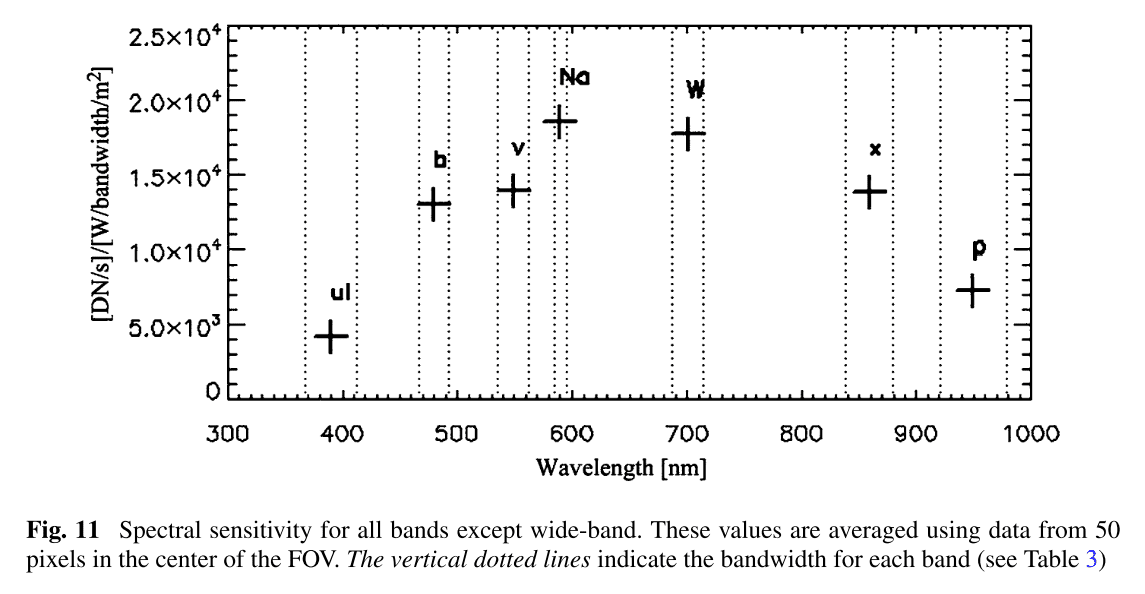
This spectral sensitivity assessment ultimately determines the signal-to-noise ratio of the imaging system, essentially how well it will be able to pick out low-intensity signals. In the case of the Hayabusa2, for example, the target asteroid’s hydrated mineral possessed a unique spectroscopic feature in the 0.7-um absorption band that the spacecraft could use for detection.

The depth of absorption of these particular minerals was only 3-4%, which meant that the visible camera had to have a high-accuracy calibration and a reasonably high signal-to-noise ratio. In this case, preflight calibration data for flat-field correction was essential, and they used a uniform light source producing the approximate spectrum and albedo anticipated from the asteroid.

In the end, the accurate calibration allowed the Hayabusa2 team to infer the absolute reflectivity of asteroids, providing invaluable scientific data for future missions.

While the Hayabusa2 team constructed their own light solution for preflight calibration, commercial tunable solar simulators are well-suited for such testing.

A few examples of different spacecraft and their primary automated navigation technologies is provided below.

Spacecraft	Agency	Mass	Cost	Propulsion	Key Tech
DART	NASA	363 kg	$95 Million	Hydrazine	AVGC (Laser Reflectance GPS Cross-Link
XSS-10	AFRL	27 kg	$100 Million	MMH / N204	VCS Relative Propagation Semi-Autonomous Behaviour
XSS-11	AFRL	138 kg	$82 Million	Hydrazine	RLS Autonomous Planner
Orbital Express	DARPA	952 kg 226 kg	$300 Million	Hydrazine	ARCSS (Cameras, Laser Ranging) AVGS Autonomous Docking

Some examples of different spacecraft and their primary automated navigation technologies. Reproduced from (Walker, 2012).

All of these missions likely benefited from good ground-testing of their instruments in advance of flight.

Solar Simulator Features that are Good for AOCS Sensor Testing

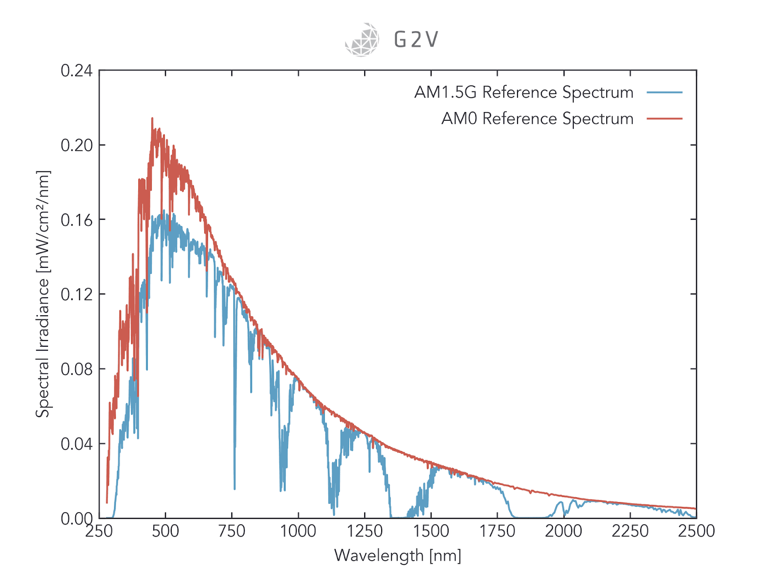
AM0 Spectrum Reproduction for AOCS Sensor Testing

Being able to produce a spectrum close to the expected spectrum in outer space (AM0) will ensure that the signal response levels of any AOCS sensor are of the appropriate magnitude.

However, one doesn’t necessarily need full spectrum reproduction for this — if the key detector is silicon-based, light outside of 350 nm – 1200 nm doesn’t really matter that much. If the detector is an RGB CCD chip, then the main spectral region of interest will be the visible range from 400 nm to 700 nm.

Therefore, while a perfect AM0 spectrum will ensure the most accurate results, getting the full spectrum can be quite costly, so comparing against your detector’s spectral response can ensure you focus on key wavelength bands of interest.

Spectral Reproduction of Stellar Object Reflectivity or Detector Response

In some cases, you might be more interested in the reflected spectrum from a stellar object, or from a star that’s not our Sun.

In those cases, a solar simulator’s tunability and flexibility in reproducing those different spectral irradiance profiles will be something to seek out to facilitate accurate test results.

For testing individual spectral bands of a visible camera, a tunable solar simulator might be most beneficial, because you can selectively turn on the spectral features of interest and be confident that there won’t be possible crosstalk or interference from neighbouring spectral bands.

G2V Optics provided a solar simulator to NASA’s Goddard Space Center for the OSAM-1 Mission for precisely this purpose.

Collimated Light for Sun Sensor Testing

Real sunlight is collimated, that is, most of the light rays are parallel to one another.

Therefore when you tilt a sun sensor in light, you’ll produce a sharp shadow, because all of the one-directional light beams will be blocked from a certain region.

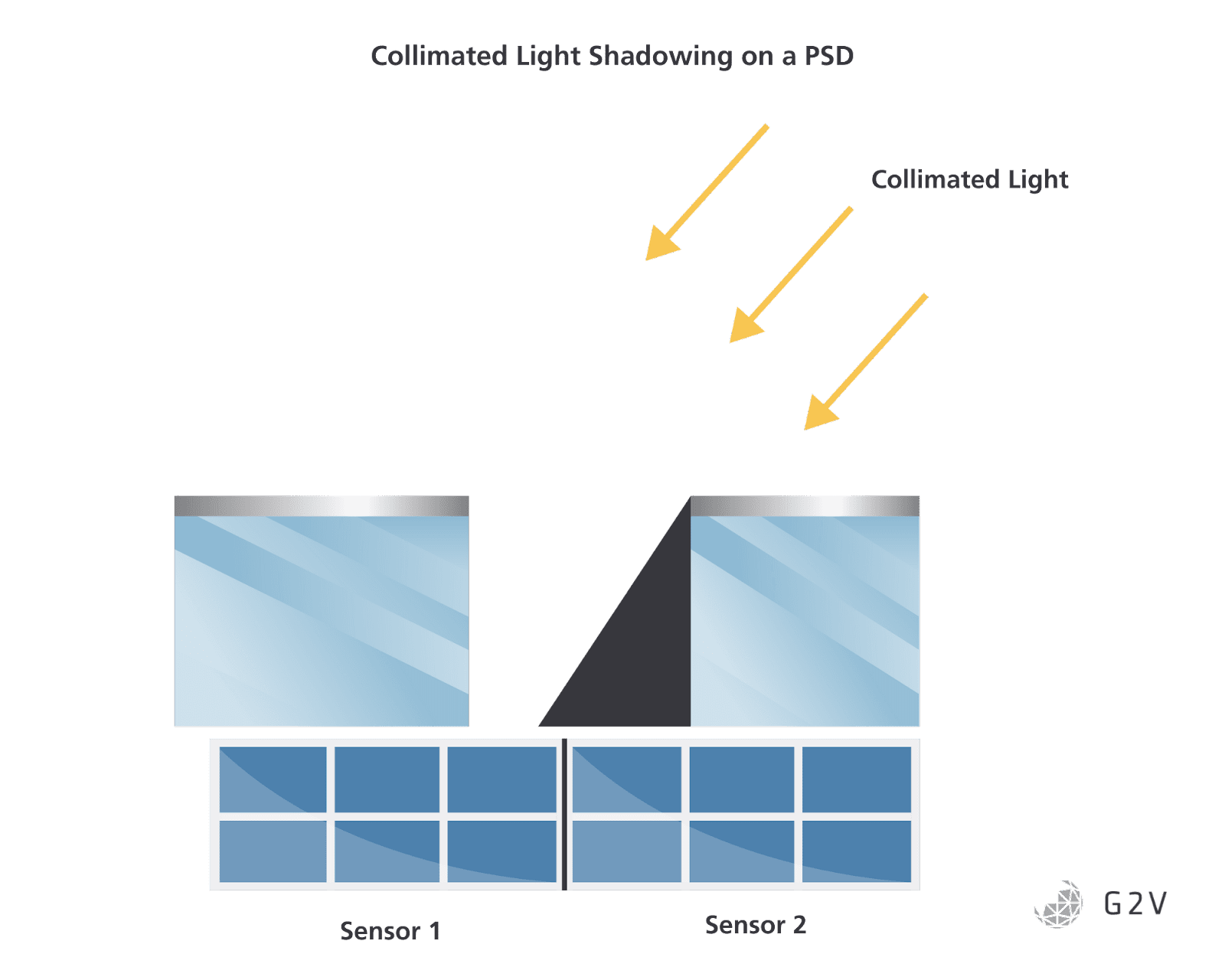
Solar simulators strive to produce collimated light, but it can be challenging from an optical design perspective.

Solar simulators will often produce a range of angular emission, and depending on the sensitivity needs of your AOCS application, that angular emission range may or may not be appropriate.

For example, a broad angular emission from a solar simulator won’t produce the same sharp shadowing effect as a collimated light source, and will therefore result in some amount of shadowing error. This may be important for a sun sensor, but less important for a visible camera that might already have a high amount of stray-light protection.

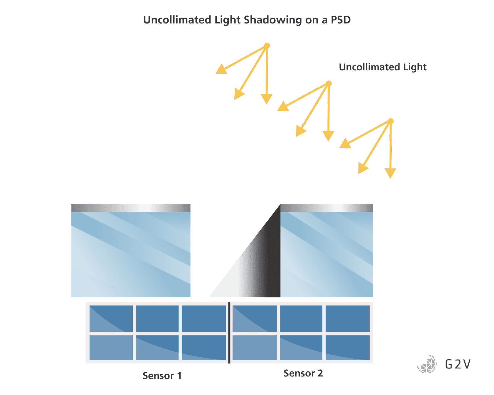
Shadowing will still occur, just with a lower precision and higher error. Many of an AOCS sensor’s behavioural trends will remain the same even when testing with a source of broad angular emission. Therefore, you’ll need to determine the allowable shadowing error and required precision for your ground tests, and select your solar simulator accordingly.

Adequate Room for Sensor Tilting

Because you’re testing your sun sensor’s angular sensitivity, you’re going to need to tilt either your light source or your sensor. Usually the sensor is much smaller than the light source, so it’s most practical to tilt the sensor.

The solar simulator’s setup and geometry need to accommodate the full range of sensor tilts you’re anticipating.

If, for example, a solar simulator is designed to be mounted above your sample, then you need to ensure the mechanical mounts of the solar simulator don’t interfere with your sample tilting, positioning and all associated apparatus. This, among many other reasons, allowed CNES to properly test their AOCS sensor using a G2V Sunbrick.

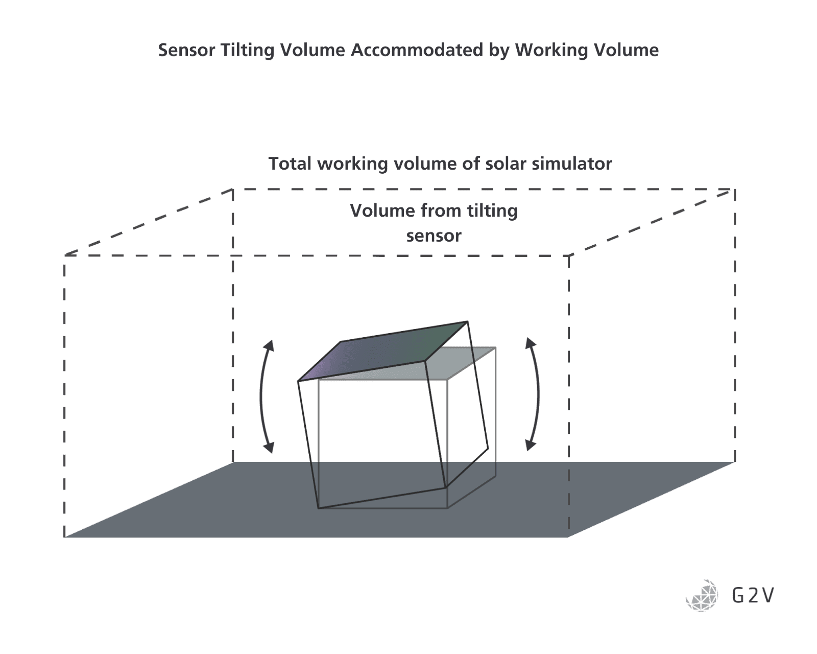
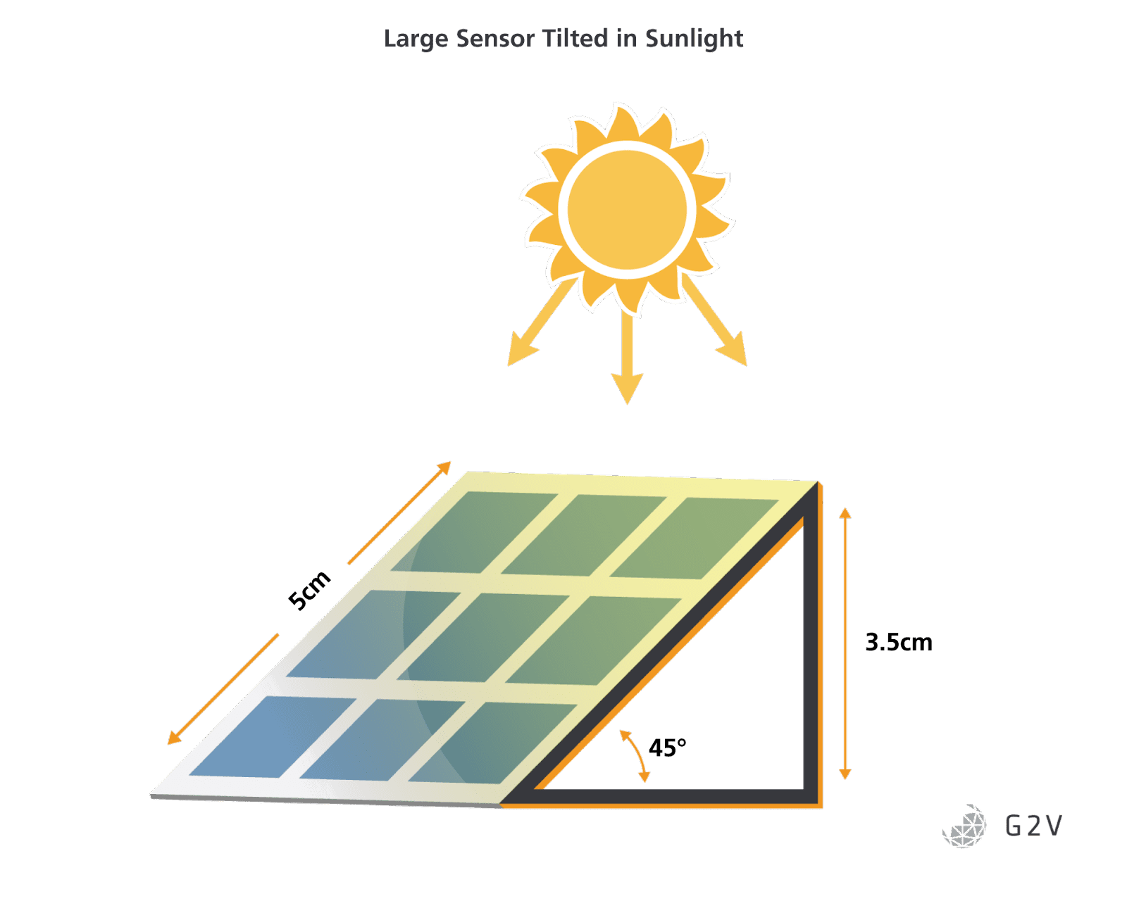
Similarly, a solar simulator must have a sufficiently large working distance to accommodate sample tilt in the first place. If, for example, you want to test up to a 45-degree tilt on a 5 cm wide sample, you can deduce from geometry that the solar simulator will need to have a working distance of at least 3.5 cm (5 cm * cos(45) = 5 cm/1.414). You know, therefore, that a solar simulator with a working distance of 1 cm is inappropriate for your testing needs.

In summary, estimate the testing volume you need based on your sample size and tilt range, and ensure your solar simulator’s mechanical configuration and working distance are appropriate.

Consistency of Irradiance with Distance

Closely related to the sensor tilt volume is how much the irradiance varies over that volume. Again, because most solar simulators do not produce perfectly collimated light, there will be a variation in intensity as a function of distance from the light source.

Usually, the intensity drops off the farther you are from the light, and the exact amount by which it drops depends on the angular collimation of the solar simulator.

You’ll need to understand the sensitivity requirements for your AOCS sensor in order to evaluate whether a solar simulator’s intensity variation with distance is acceptable or not. In some cases, you may be able to compensate for the solar simulator’s variance if you know it in advance of your analysis.

Many AOCS sun sensors have small active areas, which will minimize the effect of this error source. To illustrate its potential impact, however, let’s take two example cases of a small sensor and a large one.

Let’s say our hypothetical small sun sensor has an active area of 1 mm by 1 mm. When tilted to 45 degrees, the front edge of the sensor will be 0.7 mm closer to the light source compared to the rear edge (1*cos(45) = 1/1.414).  

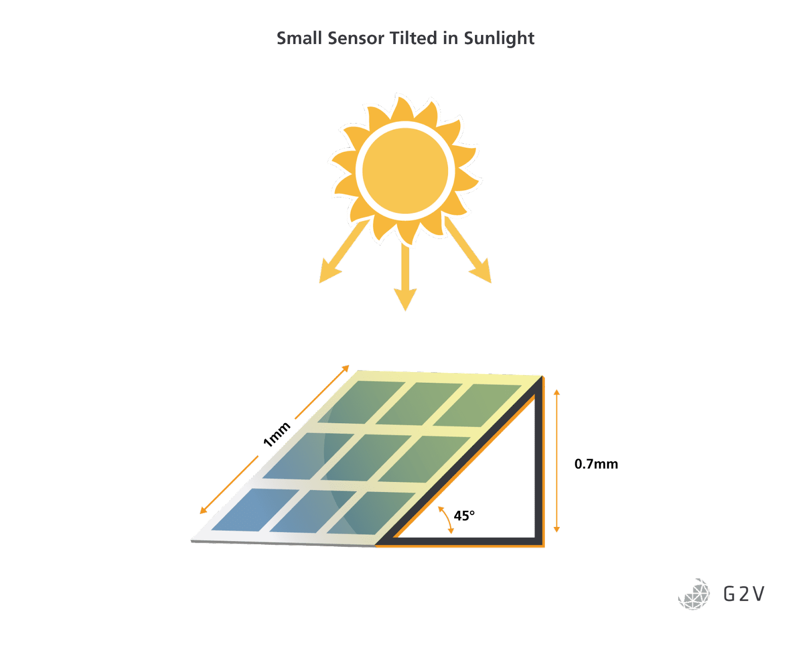
The large sun sensor, on the other hand, has an active area of 5 cm by 5 cm. When tilted to 45 degrees, the front edge of the sensor will be 3.5 cm closer to the light source compared to the rear edge (5*cos(45) = 5/1.414).

Now let’s compare these two sensors to some hypothetical solar simulator performance. In the figure below, we’ve plotted the average irradiance of two hypothetical solar simulators, each with a different falloff of irradiance as a function of working distance.  

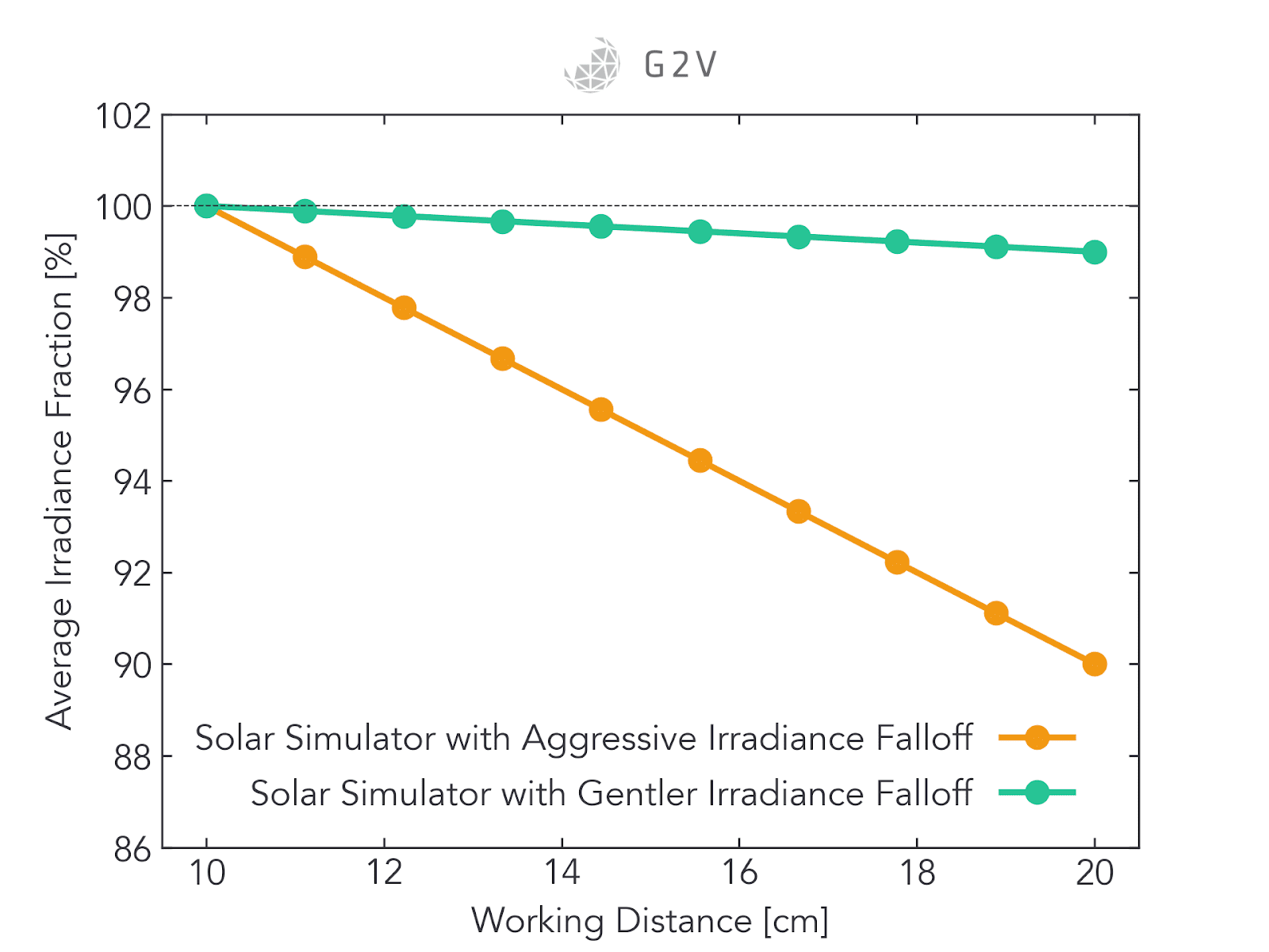
For simplicity, one solar simulator (plotted above in yellow) loses 1% of its intensity every cm. In the case of the small sensor, this means that there will be a 0.7% intensity difference between the closest and farthest edges of the sensor. It’s likely that this intensity difference is small enough to have a minimal impact on the overall shape of the AOCS sensor’s relative differential function (defined above).

The case of the large sensor is quite different, however. It will have a 3.5% intensity difference between its closest and farthest edges. This difference might be large enough that the shape of the AOCS sensor’s relative differential function (defined above) will be significantly different than what’s anticipated under collimated light conditions. In this situation, therefore, you might need either additional compensating calculations, or a solar simulator with a lower intensity drop versus distance.

The other hypothetical solar simulator (plotted above in green) that loses 0.1% every 1 cm, for example, would reduce the front-to-back variance to 0.35%, and result in a calibrated differential function much closer to reality.

While the exact criteria and cutoff values will vary depending on your specific application requirements and geometry, it’s important to consider the impact of the solar simulator’s intensity variation with distance, and whether or not the light source will be able to meet your calibration and testing requirements under the full range of expected tilt values.

A Final Word on AOCS Sensor Testing

In any aerospace application, component-level testing is important, but in space applications, it’s paramount. York University’s Space Engineering Laboratory summarizes the requirements succinctly:

“…Systems and electronics are analysed down to a component level to ensure that the failure of any particular constituent part will not jeopardise the longevity of the whole mission.”

AOCS sensors form one such subsystem must be analyzed to a deep component level, for accuracy, precision and reliability.

Knowing how to properly test these sensors on the ground in advance of flight, while compensating and being aware of solar simulator limitations and error sources, can ensure accurate sensor development in preparation for the final mission. 

For a specific example of solar simulator usage in AOCS subsystem testing, please see our case study with the French space agency CNES. Or you can check out our work on providing sunlight for testing NASA Goddard’s OSAM-1 visible camera, or our guide for how to generally test optical detectors.  

Most often, the calculation of a spacecraft’s attitude is achieved by fusing information from a variety of sensors into one trusted estimate (Space Engineering Laboratory, 2014a). Ultimately, the overall model of a space mission needs to be verified through reliable technical measures, behavioural simulations and engineering analysis (SBIR, 2022). In the following sections, we’ll go through the details of how to test some of these other aerospace sensors and subsystems in order to validate a mission model and ensure a successful flight.

Testing Visible Cameras For Aerial Imaging

One important application for sensors in the field of aerospace is in the realm of aerial imaging. Aerial imaging is done for many reasons – one of them is mapping, whether that be terrain, coastlines, ocean floors, sea-states, moons, planets or other celestial objects. Another is for monitoring city changes, vegetation, animal wildlife, clouds or even forest fires. Detailed information is required for a wide variety of conditions.

Aerial imaging falls under the umbrella of the broader term known as remote sensing, which refers to “the process of detecting and monitoring the physical characteristics of an area by measuring its reflected and emitted radiation at a distance” (US Geological Survey, 2022). Many global phenomena require accurate, continuous monitoring.

 

In the field of remote sensing for plant phenotyping alone, there are a variety of sensors used, as shown in the table below.

Sensor type	Details	Applications	Limitations
Fluorescence sensor	Passive sensing: visible and near-infrared regions	Photosynthesis, chlorophyll, water stress	Not developed for UAV research yet Can be subject to background noise
Digital camera (RGB)	Gray scale or colour images (texture analysis)	Visible properties, outer defects, greenness, growth	Limited to visual spectral bands and properties
Multispectral camera/colour-infrared camera	Few spectral bands for each pixel in visible-infrared region	Multiple plant responses to nutrient deficiency, water stress, diseases among others	Limited to few spectral bands
Hyperspectral camera	Continuous or discrete spectra for each pixel in visible-wavelength region	Plant stress, produce quality, and safety control	Image processing is challenging Sensors can be expensive
Thermal sensor/camera	Temperature of each pixel (for sensor with radiometric calibration) related to thermal infrared emissions	Stomatal conductance, plant responses to water stress and diseases	Environmental conditions affect the performance Very small temperature differences are not detectable High resolution cameras are heavier
Spectrometer	Visible near-infrared spectra averaged over a given field of view	Detecting disease, stress and crop responses	Background such as soil may affect the data quality Possibilities of spectral mixing More applicable for ground-based systems
3D camera	Infrared laser-based detection using time-of-flight information	Physical attributes such as plant height and canopy density	Lower accuracies Field applications can be limiting
LIDAR (Light Detection and Ranging) sensor	Physical measures resulting from laser (600 nm – 1000 nm)	Accurate estimates of plant/tree height and volume	Sensitive to small variations in path length
SONAR (Sound Navigation and Ranging) sensor	Sound propagation is used to detect objects based on time-of-flight	Mapping and quantification of the canopy volumes, digital control of application rates in sprayers or fertilizer spreader	Sensitivity limited by acoustic absorption, background noise, etc. Lower sampling rate than laser-based sensing

Table illustrating the variety of sensor types used for plant phenotype characterization, reproduced from https://doi.org/10.1016/j.eja.2015.07.004

In the realm of planetary surveys, the scientific searches for water and life lead to a cornucopia of instrumentation requirements and strategies, summarized in the table below.

Science Goal:
Terrain Feature of Interest	How to Evaluate	Possible Sensors and Imaging/Survey Strategies
Search for Water
Gullies	Erosion on hillsides possibly created by water	Sensitive (scanning laser) altimeter to map terrain. Imaging comparison against known classifier forms at Mars analog facilities.
Ancient River Basins	Linear ground depressions	Sensitive (radar) altimeter, mapping of terrain to find and follow possible river channel from start to finish. Image, characterize and identify terrain colour changes associated with water-modified mineral deposits.
	Chemical distributions along river bank	Onboard spectrometer to identify and map distributions
		Delivery of chemical-assay contact pods (single or long linear rope-type) to verify actual composition
	Rock distributions from large boulders to smaller rocks that would have been deposited by ancient water flow	Integration of spectrometer, altimeter, and imaging sensor data to map and recognize size and distribution of rocks.
		Vision-based assessment of terrain rockiness and distribution. Accurate delivery of small mobile robot that can image and sample rocks and boulders up close.
Water Hillside outflows	Depressions or caves in hillsides where water may have flowed out of and may still exist	Accurate navigation using prior 3D imaging of the hillsides and rivers leading to them. Sensitive forward-looking radar to image hillside to identify depressions. Forward-looking spectrometer to identify possible residual water.
		Accurate placement of tetherbot with close up spectrometer and imaging capabilities. Persistent tetherbot supports analysis across multiple seasons at this site.
Identification of water ice in glacial form	Identification of water-based glacier and terrain beneath	Downward-looking radar or Lidar to identify differences between upper surface and ground below. Spectrometer to identify water in ice and possible outflows.
		Contact drop pod that can return surface and near surface content to verify glacier.
		Deployment of subsurface penetrator pod to image and sense glacial material. Deployment of multiple persistent penetrators may provide verification of glacial drift.
Existence of subsurface water	Water located below the surface	3D mapping of surface to identify low areas. Penetrating radar or spectrometer to identify subsurface areas.
		Deployment of surface pods to characterize surface, deploy subsurface penetrator to gather imaging and chemical signatures.
Search for life
Existence in ancient lake bottoms (striated rocks)	Striated rocks on hillsides may indicate riverbeds and fossil areas	3D mapping of terrain. Imaging identification of rock areas.
Subsurface life	Recognition of chemical processes (methane, chemical signatures) identifiable on surface	Large scale search of surface for spectral signatures
		Deployment of surface imaging and contact pods
		Deployment of subsurface penetrators to image and subsurface life.

Terrain features that relate to the search for water and life, and what instruments can be used to detect them. Reproduced from https://doi.org/10.1117/12.595353

As you can probably glean, aerial imaging as part of remote sensing has wide and profound implications on humanity’s understanding of the universe we inhabit. Whether you’re looking at local vegetation or scanning cliff erosion on distant planets, you need an aerial imaging system that works with you to provide accurate data.

There are a number of challenges that can impede good aerial image capture. We’ll discuss some of them below, along with some ways that researchers and designers have overcome them.

Challenges in Aerial Imaging

Regardless of the application, aerial images require image processing. A chief concern for aerial imaging is what’s called orthorectification, when an image is converted into a suitable form by correcting distortions from sensor response, satellite/aircraft motion and terrain-related effects.

It’s ideal to test as much as possible for these types of distortions on the ground, in advance of flight.

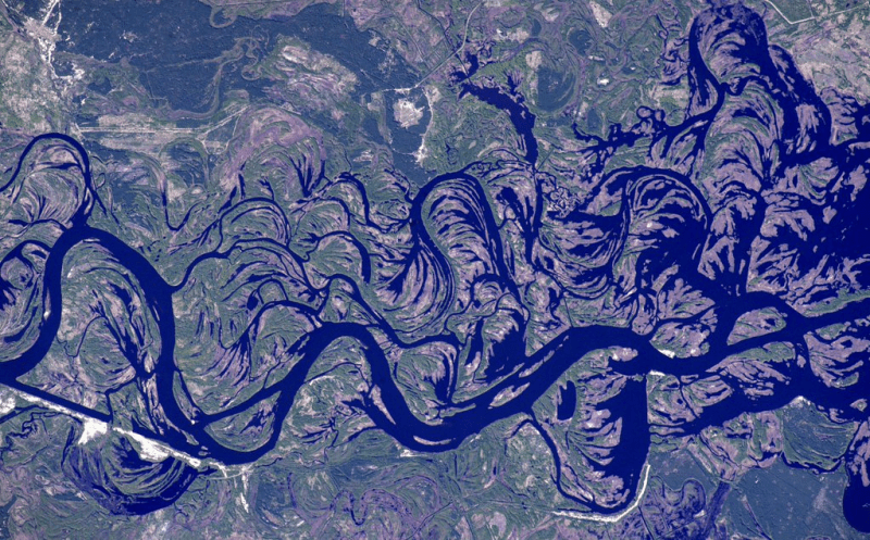
An example of orthorectification is shown below.

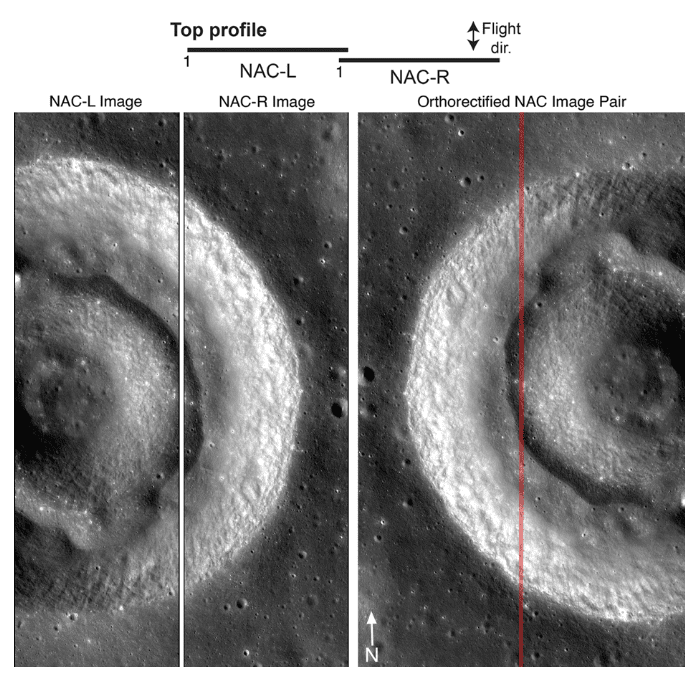
Often aerial imaging requirements can be quite demanding, pushing the technological limits of the detector, optics, and image processing techniques. For example, the Lunar Reconnaissance Orbiter aimed to have complete mapping of the Moon at pixel scales ranging from 25 cm to 200 cm.

For mapping purposes, it is most often desirable to capture nadir images — that is, images taken directly below an aircraft or spacecraft.. Off-nadir or oblique images are not as useful for map generation, but they can often reveal details that might be otherwise obscured by a strict top-down view.

Ultimately designers want to generate a camera model that fully describes an aerial imager’s behaviour under the expected flight conditions. Such camera model generation is what was done, for example, by the team developing the Lunar Reconnaissance Orbiter Camera, in order to ensure high-quality data capture during expensive missions to the moon’s orbit (Speyerer et al, 2016).

Some of the assessments required in order to build an accurate camera model include measuring bias current, dark current, field-of-view flatness, sensitivity, and the point spread function.

The Impact Of Sunlight On Bias And Dark Current Measurements

Bias current and dark current are somewhat interchangeable terms referring to the detected image or current when there is no incident light. This often informs the noise floor of the instrument and therefore the minimum detectable signal. Temperature is one factor which strongly impacts the dark current of any photodetector (including camera CCD chips).

Because aerial imaging can occur in a wide variety of weather conditions and positions relative to the Sun, the temperature of the imager, and therefore the dark current also vary according to these conditions. Understanding the complete dark current behaviour of the imager under its full range of expected temperatures is important to building an accurate camera model.

Furthermore, understanding how the Sun’s position impacts temperature variations can help a designer assess whether or not certain flight paths require additional image correction or should be avoided altogether.

A solar simulator may prove useful in assessing the temperature and dark-current dependence relative to the sun’s position.

The Impact of Sun Scatter and Clouds on Aerial Imaging

Scattering from atmospheric particulates can influence the background light level and overall cloudiness of images. Clouds themselves can also create shadows that might make accurate feature and topographical mapping challenging.

Testing Field-of-View Flatness and Sensitivity of an Aerial Imager

In any imaging system, knowing whether or not a given pixel’s brightness can be trusted is paramount. A perfect imaging system would look at a flat, uniform irradiance field and produce an equally flat image where every pixel has the same brightness.

In reality, however, every imaging system has a limited area over which it will produce a flat response, and there will be some roll-off at the edges.

Testing field-of-view flatness can be done with a uniform light source, and then the obtained flatness profile can then be used to correct any of the camera’s images in the future (forming part of the camera model).

The same type of test can be done in order to determine the pixel brightness as a function of the input intensity, otherwise known as the sensitivity. Both the sensitivity and flatness are going to vary depending on the wavelength of incident light, and they should be tested for the full spectral response range of the camera’s detector. Often designers will test imagers under the full spectrum to assess the aggregate system behaviour under expected conditions.

We provided an example of field-of-view flatness and sensitivity tests in the “Testing Visible Cameras for Orbital Maneuvers”  section above.

Shadows Challenge Automated Imaging Algorithms

Shadow poses a particular challenge for automated imaging algorithms related to vegetation. Shadows exaggerate the size of trees and shrubs, as well as causing them to smear and merge into adjacent objects, creating an illusion of movement. For many applications, it is therefore important to test an aerial imager’s (and its algorithms) ability to discern objects from their shadows. Otherwise, images have to be captured under light cloud cover to avoid generating shadows in the first place.

In some applications, however, the complete absence of shadows can make feature identification particularly challenging. There’s therefore an optimal lighting for each application, and being able to fully understand the acceptable boundaries of illuminance can ensure you capture data in the best manner.

Solar Simulator Features that are Good for Testing Aerial Imagers

Good Spatial Non-Uniformity for Evaluating Aerial Imager Field-of-View  Flatness

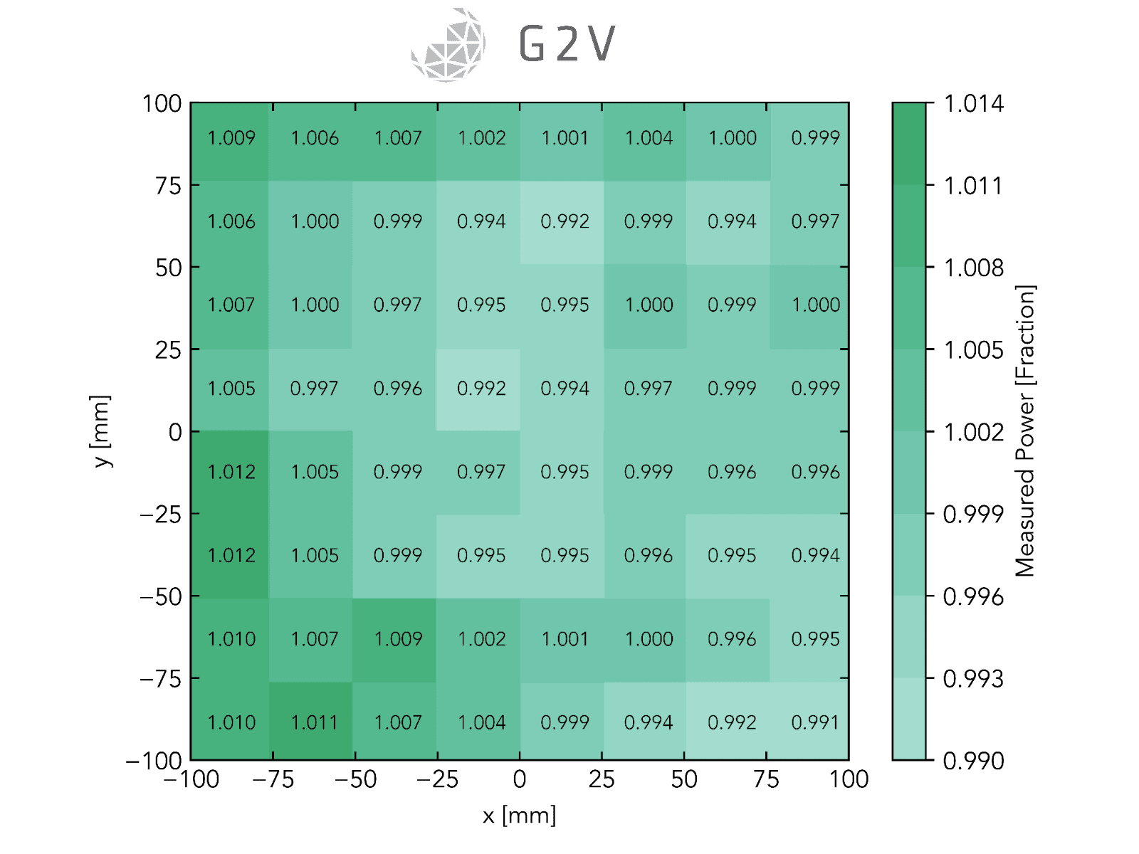
In order to assess an aerial imager’s field-of-view (FOV) flatness, you need a uniform light source. Solar simulators are required to have either Class A+ (1%), A (2%), B (5%), or C (10%) spatial non-uniformity, so this light source requirement comes as part of any solar simulator package.

An example plot of spatial non-uniformity for G2V’s Sunbrick is shown below. Ensuring that solar simulators have an acceptable non-uniformity tolerance in your intended imaging area will ensure you can accurately assess your imager’s FOV flatness.

Spectrum That Matches Detector Responsivity

You want to test your camera over the full range of imaged wavelengths, so assessing its bias current, flatness, and sensitivity for all wavelengths is vital. Getting a light source that can produce the full set of wavelengths is ideal.

Furthermore, if you want to test different camera channels (for example, red, green and blue channels in an RGB camera), the ability to selectively turn on and off desired wavelength bands can be very useful to accelerate your probing of specific camera behaviours.

This tunability is much easier to achieve with LED solar simulators than it is for traditional bulb-based solar simulators such as xenon-arc or metal-halide.

Spectrum That Matches Expected Reflectance

If you are imaging a unique surface that you know will have a peculiar reflected spectrum, it can be very useful to do your testing with a light source that can accurately mimic that reflected spectrum, so you can directly assess all your sensitivity and field of view parameters with respect to the object(s) intended for imaging. Again, LED solar simulators have a much easier time achieving this tunability than traditional bulb-based solar simulators.

IR emission to fully assess temperature effects

As mentioned above, the dark current behaviour of an aerial imager will depend on the temperature which in turn depends on the incident light. To fully reproduce the temperature changes at different angles, one would ideally have a light source that emits IR in the same manner as direct sunlight. In practice, this can be difficult to achieve, since all solar simulators will have some deviations from direct sunlight, and the solar simulator standards only specify spectral match out to 1400 nm.

In general, LED solar simulators don’t emit as far out into the IR as traditional bulb-based lamp sources such as xenon-arc or metal-halide. However, there is still variance between a bulb-based lamp’s output in the IR compared to traditional sunlight (generally, bulb-based lamps emit more IR), so be wary of relying too heavily on these temperature estimates.

Collimated Light to Accurately Mimic Shadowing 

One approach to test the effects of shadowing might be to construct a miniature diorama and then illuminate it with your own miniature sun (solar simulator). This can allow you to do initial testing on an algorithm’s ability to discern features from their shadows, for example, all in advance of flight.

For this type of testing to be accurate, however, the light source must emit mostly collimated light, which means most of the light rays must be parallel to one another. Solar simulators vary widely in this regard, so be sure to check a given solar simulator’s specifications before relying on it for this purpose.

An uncollimated light source will not produce as sharp a shadow as collimated light, and so might be misleading when trying to mimic real-life shadowing effects and their impact on imaging algorithms.

A Final Word on Aerial Imager Testing

Ground and geometric calibration of visual imagers prior to launch can make or break their eventual data collection. In the case of the Lunar Reconnaissance Orbiter Camera, the calibration prior to launch at Malin Space Science Systems in San Diego, enabled the team to determine an accurate camera model for all three onboard cameras, ultimately resulting in the accurate orthorectification of over a million images. They produced the “best georeferenced image products for cartographic studies and analysis of the lunar surface.”

The ever-increasing demands on aerospace sensors mean that they must be assessed more accurately than ever. Imagers with dual roles of navigation and science sensors must be well-understood and able to be relied upon in both roles. Implementation of increasing autonomous algorithms in these applications means an additional higher need for benchtop testing.

Some of the desired outcomes of some aerial data analysis imaging algorithms is provided below as an example of some of the directions in which the industry is moving, all of which will require extensive testing.

A wish-list of autonomous features related to aerial data analysis and image processing, reproduced from (Young et al., 2005): 

Navigation and Flight Control

• Ability to create localized maps used for navigation.
• Autonomous target and feature tracking
• Ability to close flight control around sensors sensors direct the vehicle’s flight
• Ability to fly random and intelligent random patterns.

Mission Decision-Making

• Management of resources of time, altitude, energy, communications, processing resources, deployable devices.
• Mission Management — Manages ultimate goals and decision making of mission.
• Management Of multiple science hypotheses with the ability to follow or discard as needed as the flight progresses.

Science Discovery  

• Ability to specify a science hypothesis and the process necessary to follow it, including sensors and analyses needed, possible alternatives, flight altitudes.

Data Analysis and Sensor Operation

• Sensor Data Coordination and Integration —integrates data from multiple sensors to support hypothesis following
• Creation of a three-dimensional surface topography map using multiple cameras and continuous image sequences from vehicle over-flight.
• Can recognize and return a terrain to include individual rocks.
• Sensor Operation — Operation of sensor to include pointing, focus, and generation of 2D and 3D data representations. Communicates and coordinates with Vehicle operator.
• Autonomous set up , gain/filter adjustment, and calibration/recalibration of sensors for use.
• “Pod Technician” —Manages status of pods and does any preparation of the pod.

As we’ve mentioned before, many aerospace applications and exploratory ventures require a combination of sensors. Aerial imagers often need to combine images and interpolate to create three-dimensional imagery. Aerial explorers in particular need vision, spectrometers, lidar, radar, and atmospheric-chemistry sensors.

From this list of required sensors that play a major role in safe and successful aerospace operations, we’ll look at LIDAR next.

Qualifying LIDAR instruments for remote sensing

LIDAR technology improves upon the traditional radar (radio detection and ranging) technique through the use of laser pulses instead of radio waves. LIDAR can either stand for “light detection and ranging” or “laser imaging, detection and ranging”.

In the field of remote sensing, it is also called airborne laser scanning (ALS), a name which arguably better describes what’s occurring during a LIDAR measurement.

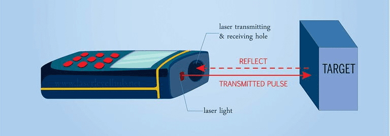
LIDAR operates by emitting a pulse or series of pulses of laser light toward a target, and then measuring the time between pulse emission and the reception of the reflected (or backscattered) signal.

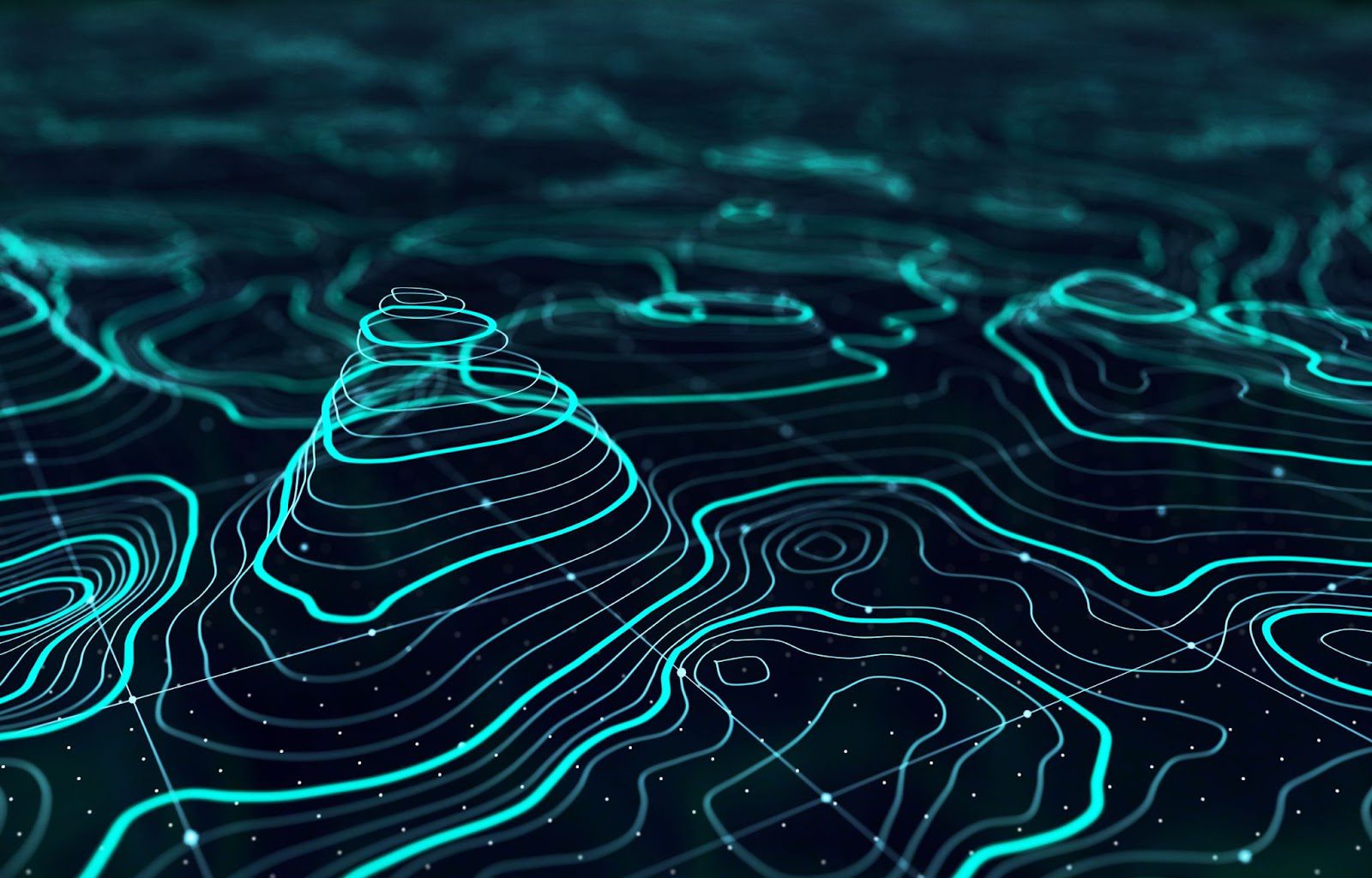
Knowing the speed of light and the direction of the laser pulse, the distance to the target can then be determined. Repeating this process over a wide area can lead to a large map of elevation and features, among other applications.

Since LIDAR uses shorter wavelengths than radar, it can detect much smaller objects and therefore has a much higher resolution. It’s a very effective technique that assists in mapping, assessing, and monitoring a wide variety of phenomena and resources, including lost cities, underwater seabeds, floods, land use, landslides, atmospheric phenomena, forests, and vegetation.

LIDAR datasets are regularly acquired over many national forests in the US. Two very broad types of LIDAR include topographic (land-mapping) and bathymetric (seafloor-mapping).

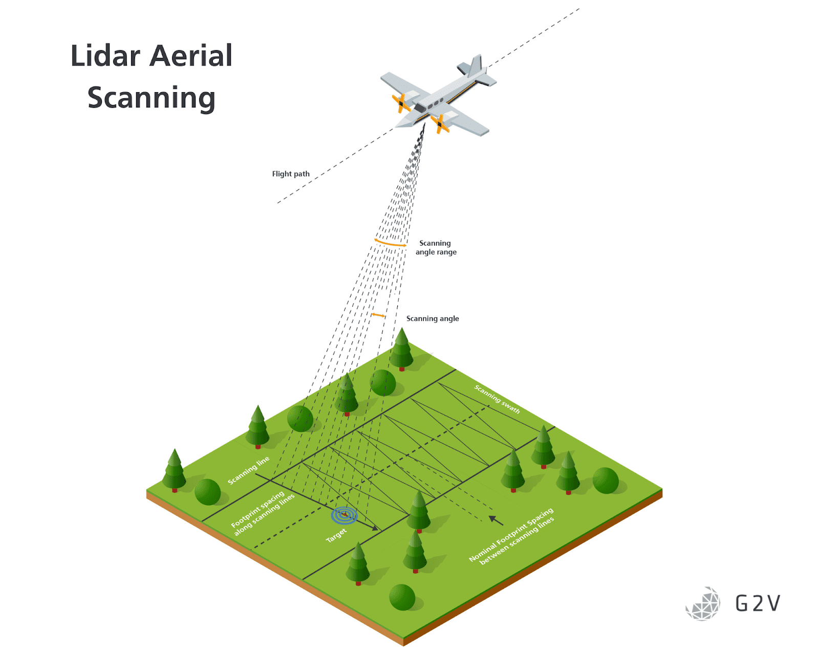
A typical LIDAR system requires more than just a laser, however. It also needs a scanning system to point the laser, an inertial navigational measurement unit (IMU) to track an aircraft’s attitude and orientation (similar to the AOCS subsystems discussed above, as well as a high-precision airborne global-positioning system (GPS) to record the three-dimensional position of the aircraft.

Finally, LIDAR generates a large amount of data, so any LIDAR system requires communication and storage devices. Often LIDAR GPS is supplemented by GPS information from a nearby ground station to correct and validate results.

A typical LIDAR measurement configuration is shown in the figure below. The scanning frequency, or number of pulses emitted per second, has grown over the years from 1,000s (1 kHz) to 100,000s (100 kHz).

The number of pulses determines the amount of so-called “discrete return signals” which can be averaged or analyzed as needed. Scanning angles are considered positive toward starboard, and negative toward the aircraft’s port side. The flight path and the scanning angle determine the scanning swath. The scanning pattern generally depends on the means by which the pulse is steered across the flight line.

As with all of the sensors we’ve discussed so far, LIDAR has advantages and limitations, and testing can greatly help mitigate its disadvantages.

Challenges with LIDAR remote sensing

The Impact of Background Light on LIDAR

LIDAR for aerial monitoring is typically carried out in the near-infrared range of 850 nm to 1060 nm, while LIDAR for bathymetric (seafloor) measurements is typically done with 532 nm (green) lasers to overcome water absorption.

Although LIDAR is emitted in a narrow bandwidth with a laser, there are still various sources that can emit in these same wavelength ranges and therefore confuse data collection.

The primary source of interference is sunlight, and its scatter and reflection off of surfaces and particulates.

Interference from sunlight can be orders of magnitude higher than weak back-scattered LIDAR signals, especially when the natural reflection of sunlight is high (such as for snow and thick clouds).

This can quickly result in detector saturation.

Even NASA’s Cloud-Aerosol LIDAR and Infrared Pathfinder Satellite Observation (CALIPSO) struggles to see very thin clouds and therefore can struggle to classify sky conditions because of sunlight interference.

The fundamental problem boils down to discriminating between a relatively weak LIDAR signal and strong sunlight scatter or reflection.

LIDAR Confusion of Pulses with Direct Reflections

Sunlight has the potential to scatter in the atmosphere to varying degrees based on particulates such as dust, water, or smog. That creates a substantial portion of the background light discussed above.

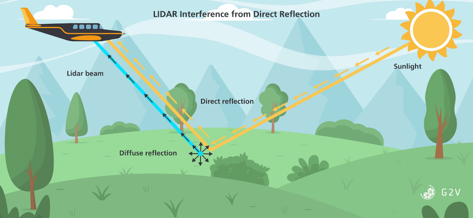
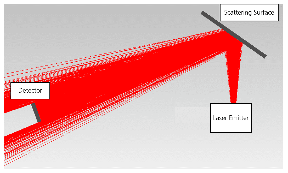
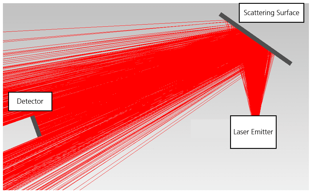
Another possible configuration for interference is via direct reflections. Certain objects of high reflectivity will shine quite brightly under sunlight and may completely drown out the LIDAR signal in certain geometries. This is particularly true for off-nadir imaging, when the LIDAR beam is moved increasingly further from the view directly below the aircraft.

The angle of incidence upon the ground increases in these situations, and the ground starts to behave more like a direct reflector than a diffuse one, so the intensity of sunlight is nearly as bright as if it were shining directly onto the detector. This is shown in the figure below.

Reflections of the LIDAR beam itself can also be problematic. Not only does direct reflection lower the intensity of the scattered LIDAR light signal, but in certain geometries direct reflection.

Therefore the range of scanning angles for a LIDAR system must be carefully selected and tested with a variety of object geometries to assess the boundary conditions where a LIDAR system will be confounded by direct ground reflection.

The removal of background sunlight interference can be achieved in several different ways. One is to use optical bandpass filters to reduce sunlight intensity. However, this technique ultimately attenuates part of the LIDAR signal as well, and so has to be executed carefully with an eye toward the fundamental signal-to-noise ratio (SNR).

Another way to overcome background sunlight is to accumulate multiple measurements and average them in order to have confidence that a given signal is not sun-contaminated. While this technique generally works, it ultimately impacts the overall framerate of a LIDAR scanner, since multiple measurements are used for a single datapoint.

A third way to overcome background sunlight is to use scanning lasers with a tighter focus, so as to raise the detected signal level well above that of the sunlight background. This approach is costly, but effective.

One group of researchers cleverly developed a photon sieve where they induced a non-zero orbital angular momentum into their output LIDAR laser pulse, then used that property during detection to differentiate between sunlight and laser light.

While there are a variety of approaches for mitigating sunlight interference, it’s an area of ongoing study where further research and testing is needed. Some of these tests may be facilitated by the use of solar simulators that can be manipulated to create different kinds of interference and scattering environments.

These types of solar simulator tests would likely need miniature dioramas or sample objects upon which to test the LIDAR interference. Because aerial LIDAR systems will have a minimum distance, the most likely setup is potentially to have a sample object or surface far away from the LIDAR instrument, and then to closely illuminate that sample object with the solar simulator.

The backscatter and reflections from the sun could then be assessed against the LIDAR signal for a variety of angles, intensities, and configurations well in advance of flight.

Wider sampling vs Data Accuracy Tradeoffs

One approach for increasing the coverage of LIDAR measurements is to use a more divergent laser beam. This increases the area sampled, and can be useful for averaging out, for example, the fine features in tree canopies that can create a lot of noise.

However, spreading the laser beam energy over a wider area results in a decrease in the overall reflected signal intensity, and can therefore lead to larger errors. A LIDAR designer has to weigh the pros and cons of their beam sampling size against their ultimate functional needs.

Another LIDAR characteristic with tradeoffs is the pulse frequency. Generally, a lower pulse frequency implies that more energy can be emitted in each pulse, because there’s more time to pump the laser’s gain medium.

However, with lower pulse frequency comes a reduced sampling rate and potentially lower scan resolution of an area. Again, the specific application details will determine the correct balance of pulse energy versus emission frequency.

For example, measuring the height of coniferous trees is much more accurate when executed with a narrow beam divergence, and high-frequency.  If you’re more interested in measuring the ground elevation, however, you may be better off with a low-frequency, wide-divergence measurement at low altitudes.

It’s important to consider these factors carefully, and it’s likely easier to test these parameters during ground tests rather than in-flight.

Biases in Ancillary Systems Causing Systematic LIDAR Errors

We’ve focused considerably on the intricacies of the optical systems in LIDAR instruments, but in reality they’re affected by every aspect of the integrated instrumentation suite. Biases or errors in the GPS, aircraft attitude, scanning angle, and pulse timing measurements can all introduce systematic errors into gathered LIDAR data.

It is important that each of these systems be tested individually and in concert with one another.

Solar Simulator Features that are Good for LIDAR Remote Sensing

Spectral Overlap With LIDAR Emitted Pulse and Detector Responsivity

When testing LIDAR systems, it almost goes without saying that a solar simulator should emit in the same detection region as your LIDAR detector and emitter. Evaluating the interference is only going to be useful in these regions.

What’s important to note, however, is that many LIDAR systems use silicon-based detectors, which, when unfiltered, will be sensitive to light in approximately the full 350 nm to 1200 nm range.

If this is the case for your LIDAR system, ensure that your solar simulator can reproduce this spectral range to test the full anticipated level of background sunlight.

Collimated Light to Ensure Accurate Angular Differentiation

The reflection, scatter and diffuse reflectance of sunlight from various surfaces will depend highly upon the incident angle of light. Since real sunlight is mostly collimated, a realistic simulation of expected conditions should be carried out with a solar simulator with as-close-to-collimated light as possible. Exactly how much collimation you require will vary depending on the application and desired test geometries. If you’re less concerned about configurations of direct reflection, then a wider-angle solar simulator might be acceptable. However, if you want to evaluate the impacts of direct reflection and unique sunlight scatter paths through forest canopies, for example, then a more collimated solar simulator is likely desirable.

Solar simulators vary widely when it comes to their output angular collimation, so be sure to check with the manufacturer to confirm it will meet your requirements. If you have a need for a highly-collimated solar simulator, we’d love to hear from you.

A Final Word on LIDAR Remote Sensing

LIDAR instrumentation is widely used for mapping a variety of phenomena on Earth and beyond. For example, the XSS-11 microsat from a US Air Force Research Laboratory used a Rendezvous Lidar System (RLS) to estimate the distance to a nearby resident space object. By “painting” the target with laser pulses, they could build a 3D model and get an understanding of its relative orientation.

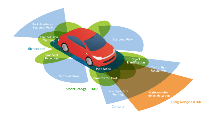
At the same time back on Earth, LIDAR technology is being increasingly used in the automotive industry, particularly for self-driving vehicles.

Overcoming the limitations of LIDAR under adverse sunlight and weather conditions can be achieved through better testing, to drive innovations and bring out unrealized potentials of the technology.

Having confidence in the measurement systems will ultimately mean more confidence in the gathered data, whether that data are in a detailed topographic map or are part of localized collision avoidance.

We’ve covered some of the main aerospace sensor types whose testing can be facilitated with solar simulators.

The applications so far have had very important roles of aircraft orientation and attitude control, visualization, navigation, and mapping.

Next, we’ll briefly discuss pyranometers which can quantify inbound radiant energy, then finish with an overview of some particularities that arise in UAV applications.

Verifying Pyranometers for Energy Quantification

Pyranometer gets its name from the Greek words pyr (fire) and ano (above), because they measure solar radiation flux. They are radiometric detectors, meaning that they use radiometric units of Joules, Watts, Watts per square meter, etc. (instead of photometric detectors that measure in human-eye-centric lux and lumens). In the aerospace industry, pyranometers are most commonly used on meteorological research aircraft with the goal of measuring upwelling and downwelling radiation.

The measured fluxes are used to characterize the reflective properties of the underlying surface, as well as cloud albedo.

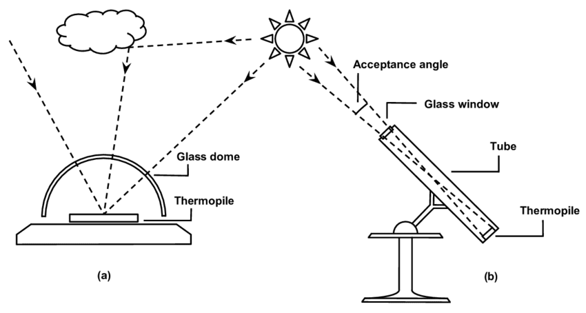
Generally, there are two broad types of pyranometers: thermopiles and silicon photocells.  

Thermopiles consist of a series of thermistors, which are electrical devices whose resistance changes quickly with temperature. Thermopiles assess inbound radiation by comparing the temperature change that radiation induces relative to a reference surface.

Silicon photocells generate electrical current through the photoelectric effect, and when calibrated with a proper solar spectrum they can be used to measure solar radiation. Silicon photocells fall under the umbrella of photovoltaics, which is a field entirely unto itself; to dive deeper, please see our comprehensive article on photovoltaics.

Outside of aerospace, pyranometers are also used in solar cell installations as part of energy monitoring and power budget estimates, in order to ensure that a given system is operating at its expected efficiency.

Maintaining calibrated pyranometers is considered by some to be an essential part of solar energy’s future, for ongoing monitoring and maintenance.

In aerospace, pyranometers are expected to continue to be used for radiative data capture, and such data can be used to predict structural insulation requirements, to find the ideal locations for greenhouses, to design commercial solar energy installations, and to study climate and meteorological effects.

Pyranometers are calibrated according to ISO 9847, and achieving good calibration can be a challenge for the particular needs of aerospace applications.

Challenges for Pyranometer Use in Aerospace

Correcting Pyranometers for Tilt and Zenith Angle

Knowing a pyranometer’s angular relationship to the measured light source is essential for accurate quantification of radiation, since a tilt relative to a source will decrease the measured amount by the cosine of the angle. Furthermore, usually aerial pyranometer measurements need to be corrected so they represent the radiation normal to the Earth’s surface.

There are then two angular components that need to be considered: the tilt of the pyranometer relative to the Sun, and the angle of the sun relative to the Earth’s surface normal.

Correctly identifying these two angles may require some additional sensors such as a sun tracker discussed in the AOCS section above.

Correcting Pyranometers for Diffuse Versus Direct Radiation

The angular corrections mentioned above generally assume direct radiation — that is, collimated light coming from a faraway source (the Sun).

However, in reality there are various types of scattering occurring in the atmosphere: isotropic scattering from aerosols, and Rayleigh scattering off of air molecules. This scattering results in varying levels of what’s called diffuse radiation to be present at any given sunlit time.

Scientists have calculated the degree of direct versus diffuse light under various Sun zenith angles and scattering models, so an approximate correction factor can be applied if the Sun’s zenith angle is known.

Solar Simulators Features that are Good for Aerial Pyranometer Testing

Known and Reliable Angular Distribution for Accurate Pyranometer Calibration

Using a solar simulator for pyranometer calibration generally reduces the error and improves accuracy compared to outdoor measurements.

However, with a solar simulator, the angular distribution of light is quite often not the same as sunlight — that is, it is not collimated, and even when diffuse light is considered, the angular profiles are still quite different.

Some pyranometers come with cosine correctors that can mitigate the dependence on angular distribution, lowering the impact of this angular profile difference.

It is therefore prudent to use a solar simulator whose angular distribution is known. While it is possible to measure this independently and derive it, a solar simulator who can provide this data for you will allow you to move quickly to pyranometer calibration instead of spending time and resources on solar simulator characterization.

Excellent Spectral Match to Ensure Accurate Aggregated Pyranometer Response

A pyranometer, whether a thermopile or a silicon photocell, is going to be measuring sunlight.

Having a solar simulator that has an excellent spectral match in most if not all of the spectral response range of your detector is vital to ensure you accurately test the full aggregate behaviour of all incident wavelengths, to the same extent the detector will experience under real sunlight.

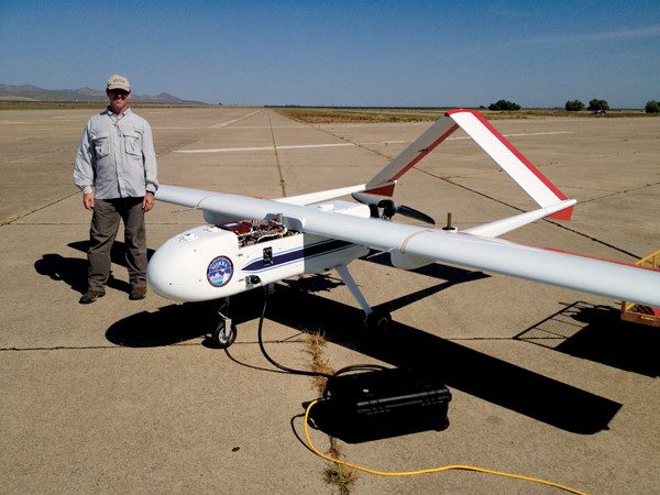
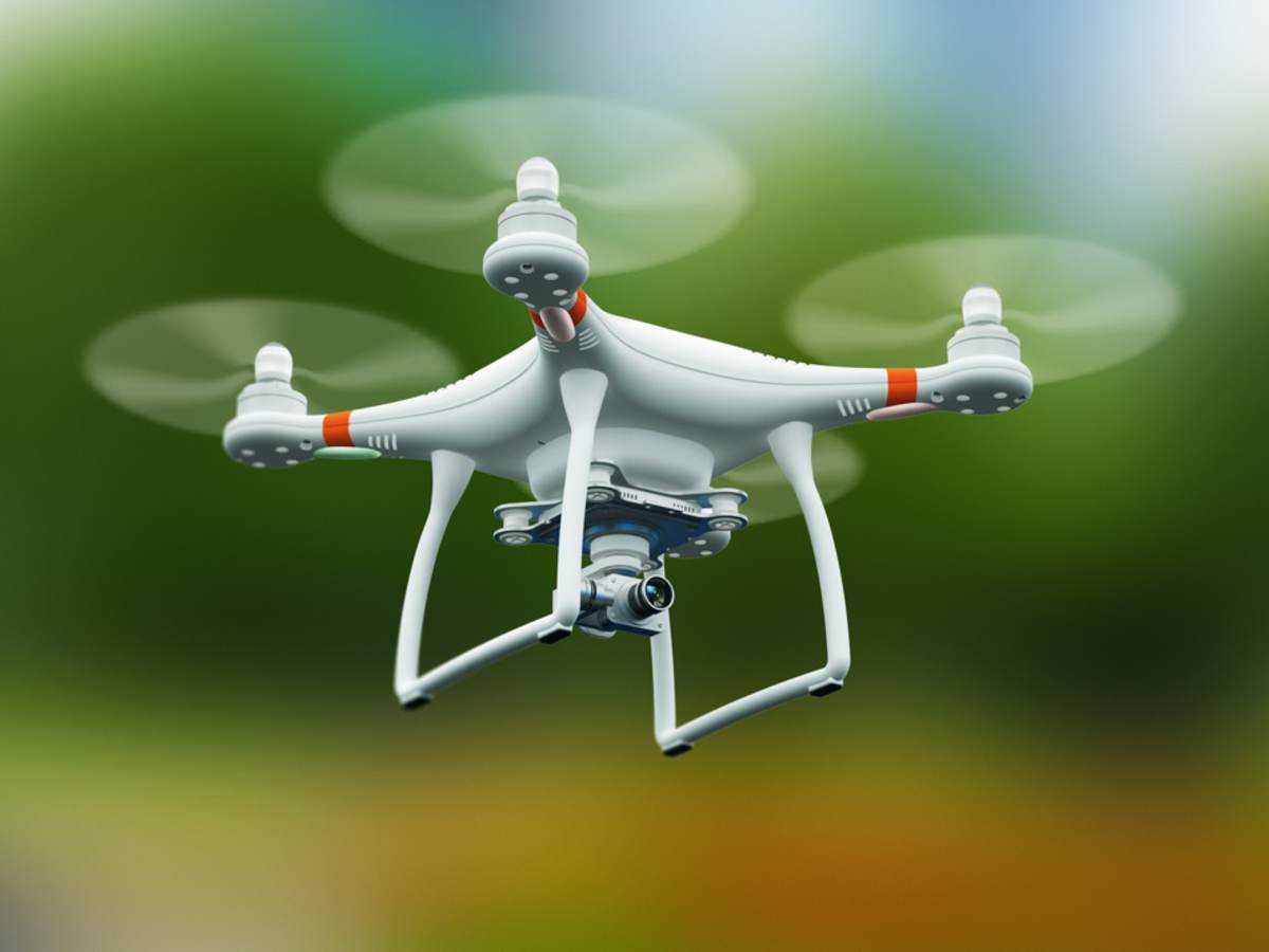
Instrumentation Requirements for UAV Applications

Unmanned Aerial Vehicles (UAVs) are a class of aircraft that have been steadily rising in popularity and usage for a wide variety of applications.

Referring to autonomous or remotely controlled aircraft, UAVs don’t have the same rigid requirements for life support and design safety, and so offer more affordable, flexible means to get instruments into the air.

Many of the same driving factors for general aerospace instrument applications also apply to UAVs, but some of the particular points of emphasis differ. Weight considerations are even more important in UAV applications, for example, driving even harder toward fewer, lighter instruments.

Another nuance is that UAVs generally fly at lower altitudes than traditional aircraft, so the sensors need to be appropriately tuned and calibrated for these regimes.

Low-altitude image data can be distorted by the same factors we’ve discussed in the Aerial Imaging section above, but because a UAV camera will “see” a much smaller portion of the Earth, they’re much more sensitive to Sun position and shadowing effects.

Because UAVs are so nimble, their platform also tilts more rapidly than traditional aircraft. This can result in more significant platform tilt distortion depending on the sensor.  

One major advantage of UAVs, however, is that they are able to safely fly much lower than manned aircraft. They’re expected to be able to measure radiative flux, topography, sea wave profiles, and wave breaking kinematics in ways that are much more challenging for traditional aircraft.

More localized phenomenological studies can be done, such as monitoring the evolution of the atmospheric boundary layer over transition zones such as air–sea ice boundaries or across sea surface temperature fronts.

Solar Simulator Features that are Good for UAV Sensor Testing

As with all of the instrumentation we’ve discussed so far, the required testing ultimately depends on the type of sensor and its intended application.

Since UAV applications to-date have been using many of the same sensors as traditional aviation, most of the advice provided in the previous sections applies with regards to sun sensors, visible cameras, LIDAR, and pyranometers.

One possible feature that might be unique to UAVs relates to their capacity for rapid tilting and possible tumbling.

Depending on the rate of a UAV sensors’ data capture, being able to correct for motion blur and platform tilt may be important.

Alongside that will come the associated need for correcting for sunlight interference under these rapid-motion conditions. It’s unlikely that a solar simulator will be able to tumble around the sensor; therefore, to simulate these conditions, a tumbling setup for the sensor itself is likely required.

Ensuring that your solar simulator can accommodate the volumetric requirements of your tumbling setup will be important for such testing.

Aerospace Sensor Testing – TL;DR

• Sensor requirements are increasing as flights reach farther and have more complex mission requirements
• Individual and integrated sensor testing in advance of flight is essential for guaranteeing mission success while minimizing development costs
• A wide variety of sensor types come with an equally varied set of testing needs, many of which require sunlight replication
• Attitude and Orbital Control Subsystems (AOCS) require solar simulators that can reproduce AM0, that can be tuned to a desired stellar reflectance profile, that are collimated for accurate star tracker testing, and that have adequate volume and irradiance behaviour for a tilted sensor’s volume
• Visible cameras for aerial imaging require solar simulators that have good spatial non-uniformity for evaluating FOV flatness, good spectral match relative to the detector responsivity or anticipated reflectance, reasonable IR emission to fully assess temperature effects, and collimated light for accurate shadow simulation.
• Aerial LIDAR instruments require solar simulators that overlap with a LIDAR’s pulse wavelength and detection wavelengths, and are collimated to enable accurate differentiation between the sunlight and a pulse
• Aerial Pyranometer instruments require solar simulators that have an excellent spectral match to sunlight and known angular light distributions that can allow for accurate diffuse versus direct light corrections.
• UAV instruments have even stricter weight requirements and require solar simulator properties similar to all the other categories, with the possible unique requirement of extra volume for testing the rapid tumbling motions expected in this aircraft.

If you have a need for a highly-collimated solar simulator, we’d love to chat and discuss your requirements

References

Beer M, Haase JF, Ruskowski J, and Kokozinski R. (2018) Background Light Rejection in SPAD-Based LiDAR Sensors by Adaptive Photon Coincidence Detection. Sensors 18(12): 4338.https://doi.org/10.3390/s18124338

Boers, R., Mitchell, R.M., and Krummel, P.B. (1998). Correction of aircraft pyranometer measurements for diffuse radiance and alignment errors. Journal of Geophysical Research: Atmospheres 103 (D13), 16753-16758. https://doi.org/10.1029/98JD01431

Bruco Integrated Circuits (2022, July 26). LIDAR – LIGHT DETECTION AND RANGING, OF LASER IMAGING DETECTION AND RANGING. Use Cases in More Detail

https://bruco-ic.com/use-cases/lidar-light-detection-and-ranging-of-laser-imaging-detection-and-ranging

Custom Control Sensors (2020, August 7). “The Future Scope of Pressure Sensors in the Aerospace Industry.” Leading Pressure & Temperature Sensing Technology | CCS DualSnap. https://www.ccsdualsnap.com/the-future-scope-of-pressure-sensors-in-the-aerospace-industry/

DARPA, (2022, November 28). Orbital Express. https://www.darpa.mil/about-us/timeline/orbital-express

Davis, T.M., Baker, T.L., Belchak, T.A., Larsen, W.R. (2003). XSS-10 Micro-Satellite Flight Demonstration Program. 17th Annual AIAA/USU Conference on Small Satellites. https://digitalcommons.usu.edu/smallsat/2003/All2003/25/

Elaksher, A.F. (2008). Fusion of hyperspectral images and lidar-based dems for coastal mapping. Optics and Lasers in Engineering 46 (7), 493-498. https://doi.org/10.1016/j.optlaseng.2008.01.012

European Union Satellite Centre (2022, July 26). Space Situational Awareness (SSA). https://www.satcen.europa.eu/page/ssa

Fensham R. J. Fairfax R. J. (2002) Aerial photography for assessing vegetation change: a review of applications and the relevance of findings for Australian vegetation history. Australian Journal of Botany 50, 415-429. https://doi.org/10.1071/BT01032

Flyguys (2022, July 26). LiDAR vs RADAR: What’s the Difference? Flyguys Nationwide Drone Services. https://flyguys.com/lidar-vs-radar/

Gatziolis, D., & Andersen, H.-E. (2008). A guide to LIDAR data acquisition and processing for the forests of the Pacific Northwest. Gen. Tech. Rep. PNW-GTR-768. U.S. Department of Agriculture, Forest Service, Pacific Northwest Research Station. https://doi.org/10.2737/PNW-GTR-768

GISGeography (2022, June 6). 15 LiDAR Uses and Applications. GIS Career.

https://gisgeography.com/lidar-uses-applications/

Guilmartin, J. F. (2022, July 26). Unmanned aerial vehicle. Britannica. https://www.britannica.com/technology/unmanned-aerial-vehicle

Hinckley, A. (2017, June 14). Pyranometers: What You Need to Know. Campbell Scientific.

https://www.campbellsci.ca/blog/pyranometers-need-to-know

Kameda, S., Suzuki, H., Takamatsu, T. et al. (2017) Preflight Calibration Test Results for Optical Navigation Camera Telescope (ONC-T) Onboard the Hayabusa2 Spacecraft. Space Sci Rev 208, 17–31. https://doi.org/10.1007/s11214-015-0227-y

Kaur, Kalwinder (2013). “What is a Pyranometer?” Azo Sensors. https://www.azosensors.com/article.aspx?ArticleID=248

Kebes (2022, July 26). File:Absorption spectrum of liquid water.png. Wikimedia Commons. https://commons.wikimedia.org/wiki/File:Absorption_spectrum_of_liquid_water.png

Liebe, C.C., Murphy, N., Dorsky, L. & Udomkesmalee, N. (2016). Three-axis sun sensor for attitude determination. IEEE Aerospace and Electronic Systems Magazine 31 (6), 6-11. https://doi.org/10.1109/MAES.2016.150024

Mariottini, F., Betts, T., Belluardo, G. (2019). Uncertainty in calibration and characterisation of pyranometers. Loughborough University. PVSAT-15 Conference contribution. https://hdl.handle.net/2134/37804

Maxar (2022, July 26). A Unique Perspective: How off-nadir imagery provides information and insight. https://explore.maxar.com/Imagery-Leadership-off-nadir

Mithrush, R. (2017, August 11). Solar Energy in India and the Importance of Pyranometer Calibration. Campbell Scientific.

https://www.campbellsci.ca/blog/solar-energy-in-india-and-the-importance-of-pyranometer-calibration

Muller, R. (2022, July 26). Orthorectification. Earth Observation Center.

https://www.dlr.de/eoc/en/desktopdefault.aspx/tabid-6144/10056_read-20918/

National Ocean Service (2022, July 26). What is lidar? National Oceanic and Atmospheric Administration. https://oceanservice.noaa.gov/facts/lidar.html

Natural Resources Canada (2016, March 2). Interactions with the Atmosphere. Government of Canada.

https://www.nrcan.gc.ca/maps-tools-publications/satellite-imagery-air-photos/remote-sensing-tutorials/introduction/interactions-atmosphere/14635

Ortega, P., Lopez-Rodriguez, G. Ricart, J. et al. (2010). A Miniaturized Two Axis Sun Sensor for Attitude Control of Nano-Satellites. IEEE Sensors Journal 10 (10), 1623-1632. https://doi.org/10.1109/JSEN.2010.2047104

Paschotta, R. (2022, July 26). Dark Current. RP Photonics Encyclopedia. https://www.rp-photonics.com/dark_current.html

Paschotta, R. (2022, July 26). Position-sensitive Detectors. RP Photonics Encyclopedia. https://www.rp-photonics.com/position_sensitive_detectors.html

PCB Piezotronics (2022, August 8). Aerospace Ground Testing. Sensors for Aerospace & Defense. https://www.pcb.com/applications/aerospace-defense/ground-testing

Porras-Hermoso A, Alfonso-Corcuera D, Piqueras J, Roibás-Millán E, Cubas J, Pérez-Álvarez J, Pindado S. (2021). Design, Ground Testing and On-Orbit Performance of a Sun Sensor Based on COTS Photodiodes for the UPMSat-2 Satellite. Sensors 21(14):4905. https://doi.org/10.3390/s21144905

Port, J. (2022, January 11). LIDAR: how self-driving cards ‘see’ where they’re going. Cosmos Magazine.  

https://cosmosmagazine.com/technology/lidar-how-self-driving-cars-see/

Reineman, B. D., Lenain, L., Statom, N. M., & Melville, W. K. (2013). Development and Testing of Instrumentation for UAV-Based Flux Measurements within Terrestrial and Marine Atmospheric Boundary Layers, Journal of Atmospheric and Oceanic Technology, 30(7), 1295-1319. https://doi.org/10.1175/JTECH-D-12-00176.1

Sankaran, S., Khot, L.R., Espinoza, C.Z. et al. (2015). Low-altitude, high-resolution aerial imaging systems for row and field crop phenotyping: A review. European Journal of Agronomy 70, 112-123. https://doi.org/10.1016/j.eja.2015.07.004

SBIR (2022, July 26). METIS: A System and MBSE Methodology for Small Spacecraft Development. US Government Small Business Innovation Research. https://www.sbir.gov/sbirsearch/detail/1670967

Scanifly (2022, July 26). What is the difference between NADIR Images and Oblique Images. Guides. https://support.scanifly.com/docs/oblique-vs-nadir-images

Sekrecka A, Wierzbicki D, and Kedzierski M. (2020). Influence of the Sun Position and Platform Orientation on the Quality of Imagery Obtained from Unmanned Aerial Vehicles. Remote Sensing 12(6):1040. https://doi.org/10.3390/rs12061040

Sheridan, K.F. (2001). GPS based position and attitude determination for airborne remote sensing. Doctoral thesis (Ph.D), UCL (University College London). https://discovery.ucl.ac.uk/id/eprint/10108272/

Space Engineering Laboratory (2014). Attitude Determination Subsystem. York University’s Space Engineering Laboratory. http://www.yorku.ca/bquine/pages/attitude_determination_subsystem.htm

Space Engineering Laboratory (2014). Background to the Spacecraft Industry. York University’s Space Engineering Laboratory.

http://www.yorku.ca/bquine/pages/background_to_space_ind.htm

Space Engineering Laboratory (2014). Mission Costs and Reliability. York University’s Space Engineering Laboratory.

http://www.yorku.ca/bquine/pages/mission_costs_and_reliability.htm

Space Engineering Laboratory (2014). Spacecraft Systems. York University’s Space Engineering Laboratory.

http://www.yorku.ca/bquine/pages/spacecraft_systems.htm

Speyerer, E.J., Wagner, R.V., Robinson, M.S. et al. (2016). Pre-flight and On-orbit Geometric Calibration of the Lunar Reconnaissance Orbiter Camera. Space Sci Rev 200, 357–392. https://doi.org/10.1007/s11214-014-0073-3

Sun, W., Hu, Y., MacDonnell, D.G., Weimer, C., & Baize, R.R. (2016). Technique to separate lidar signal and sunlight. Opt. Express 24, 12949-12954. https://doi.org/10.1364/OE.24.012949

Swank, A.J., Aretskin-Hariton, E., Le. D.K., and Sands, O.S. (2017). Beaconless Pointing for Deep-Space Optical Communication. AIAA International Communications Satellite Systems Conference Proceedings. https://ntrs.nasa.gov/citations/20170001298

US Geological Survey (2022, July 26). What is remote sensing and what is it used for?

https://www.usgs.gov/faqs/what-remote-sensing-and-what-it-used

Walker, L. (2012). Automated Proximity Operations Using Image-Based Relative Navigation. Proceedings of the Small Satellite Conference, Session VIII: Frank J. Redd Student Scholarship Competition, 3. https://digitalcommons.usu.edu/smallsat/2012/all2012/65/

Walker, P. M., & Trexler, D. T. (1977). Low sun-angle photography. Photogrammetric Engineering and Remote Sensing 43, 493-505. https://www.asprs.org/wp-content/uploads/pers/1977journal/apr/1977_apr_493-505.pdf

Wall, M. (2021 November 15). “Kessler Syndrome and the space debris problem.” Space.com. https://www.space.com/kessler-syndrome-space-debris

Wei, X., Zhang, G., Fan, Q., Jiang, J., & Li, J. (2014). Star sensor calibration based on integrated modelling with intrinsic and extrinsic parameters. Measurement 55, 117-125.

https://doi.org/10.1016/j.measurement.2014.04.026

Wikipedia (2022, July 26). Radar. https://en.wikipedia.org/wiki/Radar

Woods Hole Coastal and Marine Science Center (2018, September 24). Aerial Imaging and Mapping. US Geological Survey. https://www.usgs.gov/centers/whcmsc/science/aerial-imaging-and-mapping

Young, L.A., Pisanich, G., Ippolito, C., & Alena, R. (2005). Aerial vehicle surveys of other planetary atmospheres and surfaces: imaging, remote-sensing, and autonomy technology requirements. Proc. SPIE 5671, Real-Time Imaging IX. https://doi.org/10.1117/12.595353